library(tidyverse)
library(patchwork)
# BiocManager::install(c("SingleCellExperiment","SingleR","celldex"),ask=F)
library(viridis)
library(Seurat)
# Anotacion de tipos celulares
library(SingleCellExperiment)
library(SingleR)
library(celldex)
# Expresion diferencial
library(edgeR)
library(RColorBrewer)
# trayetcoria
library(plotly) # figura interactiva
options(rgl.printRglwidget = TRUE)
library(sparseMatrixStats)
library(slingshot) # BiocManager::install("slingshot")
library(tradeSeq) # BiocManager::install("tradeSeq")
library(Matrix)Práctica 4: COVID-19 vs healhty
Descripción de los datos
Información general
- Título del estudio: Immunophenotyping of COVID-19 and Influenza Underscores the Association of Type I IFN Response in Severe COVID-19
- Especie: Homo sapiens
- Número de acceso de la base de datos GEO (Gene Expression Omnibus): GSE149689
- Tipo de experimento: scRNA-seq
Paso 1. Cargar paquetes y datasets en R
Cargar paquetes
Cargar el dataset de pbmc_integrated
Objetos obtenidos de de la Practica 2.
# Cargar el objeto desde el archivo RDS
pbmc_integrated <- readRDS("output/pbmc3k_integrated.rds")

# Unir las capas del assay activo (ej. RNA)
pbmc_integrated <- JoinLayers(pbmc_integrated)

# convertir de objeto seurat a SingleCellExperiment
sce <- as.SingleCellExperiment(pbmc_integrated)

# descargar referencia de human cell atlas
ref.set <- celldex::HumanPrimaryCellAtlasData()

# Set the identity as louvain with resolution 0.5
sel.clust <- "RNA_snn_res.0.5"
# La identidad activa (active.ident) es la variable que Seurat usa por defecto para agrupar células en funciones como FindMarkers, DimPlot, etc
alldata <- SetIdent(pbmc_integrated, value = sel.clust)
# Número de células en cada cluster
table(alldata@active.ident)
  0   1   2   3   4   5   6   7   8
622 620 420 327 179 147 122  88  23
Paso 2. Asignar identidad celular a los clusters (SingleR + celldex)
Ahora etiquetaremos nuestras células utilizando el objeto `SingleCellExperiment`, con la referencia establecida anteriormente.
pred_main <- SingleR::SingleR(test = sce,
                              ref = ref.set,
                              labels = ref.set$label.main)

pred_fine <- SingleR::SingleR(test = sce,
                           ref = ref.set,
                           labels = ref.set$label.fine)
Conserva los tipos que tengan más de 10 celdas en la etiqueta, vuelve a asignar esas etiquetas a nuestro objeto Seurat y visualízalas en nuestro umap.
lbls.keep <- table(pred_main$labels) > 10

pbmc_annotated <- pbmc_integrated
pbmc_annotated$SingleR.labels <- ifelse(lbls.keep[pred_main$labels], pred_main$labels, 'Other')

DimPlot(pbmc_annotated, reduction='umap', group.by='SingleR.labels')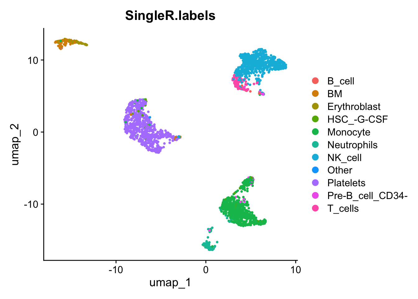
Es bueno ver que, aunque SingleR no utiliza los clústeres que calculamos anteriormente, las etiquetas parecen coincidir bastante bien con esos clústeres.
How many cells have low confidence labels?
unique(pred_main$pruned.labels) [1] "Platelets" "CMP" "Monocyte" "BM"
[5] "Erythroblast" "Neutrophils" "NK_cell" NA
[9] "HSC_-G-CSF" "Pre-B_cell_CD34-" "T_cells" "Pro-B_cell_CD34+"
[13] "B_cell" "Macrophage" # Opción A
table(pred_main$pruned.labels)
          B_cell               BM              CMP     Erythroblast
              14               86                3               64
      HSC_-G-CSF       Macrophage         Monocyte      Neutrophils
              37                1              645              120
         NK_cell        Platelets Pre-B_cell_CD34- Pro-B_cell_CD34+
             638              707               19                1
         T_cells
              95
# Opción B
table(pred_main$labels)
          B_cell               BM              CMP     Erythroblast
              14               87                3               64
      HSC_-G-CSF       Macrophage         Monocyte      Neutrophils
              37                1              723              121
         NK_cell        Platelets Pre-B_cell_CD34- Pro-B_cell_CD34+
             669              707               19                1
         T_cells
102 summary(is.na(pred_main$pruned.labels)) Mode FALSE TRUE
logical 2430 118 Are there more or less pruned labels for the fine labels?
summary(is.na(pred_fine$pruned.labels)) Mode FALSE TRUE
logical 2448 100 Now that we understand what the singleR dataframe looks like and what the data contains, let’s begin to visualize the data.
plotDeltaDistribution(pred_main, ncol = 4, dots.on.top = FALSE)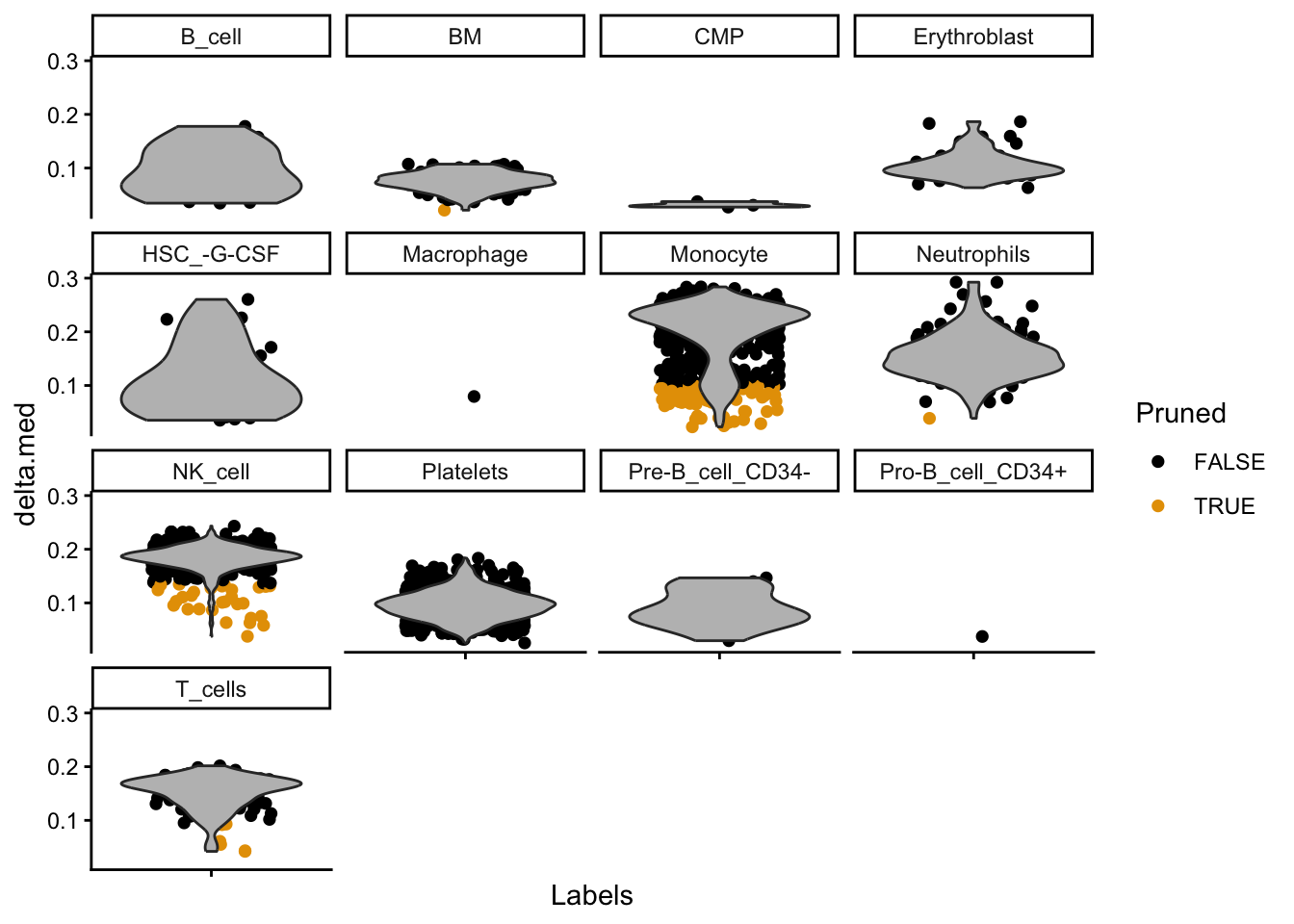
plotScoreHeatmap(pred_main)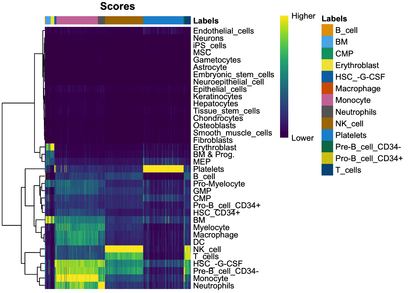
Rather than only working with the singleR dataframe, we can add the labels to our Seurat data object as a metadata field, so let’s add the cell type labels to our seurat object.
#add main labels to object
pbmc_annotated[['immgen_singler_main']] = rep('NA', ncol(pbmc_annotated))
pbmc_annotated$immgen_singler_main[rownames(pred_main)] = pred_main$labels

#add fine labels to object
pbmc_annotated[['immgen_singler_fine']] = rep('NA', ncol(pbmc_annotated))
pbmc_annotated$immgen_singler_fine[rownames(pred_fine)] = pred_fine$labels
Comparing the labels obtained from the three sources, we can see many interesting discrepancies. Sorthing those out requires manual curation. However, many informative assignments can be seen. For example, small cluster 17 is repeatedly identified as plasma B cells. This distinct subpopulation displays markers such as CD38 and CD59.
FeaturePlot(pbmc_annotated, "CD38") + scale_colour_gradientn(colours = rev(brewer.pal(n = 11, name = "Spectral")))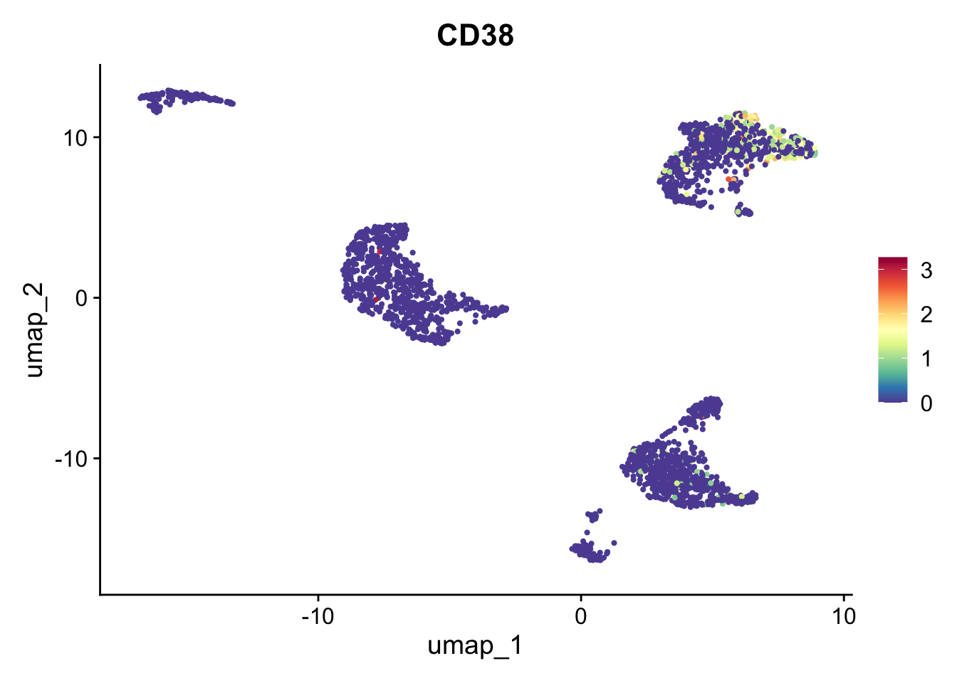
Similarly, cluster 13 is identified to be MAIT cells. Literature suggests that blood MAIT cells are characterized by high expression of CD161 (KLRB1), and chemokines like CXCR6. This indeed seems to be the case; however, this cell type is harder to evaluate.
FeaturePlot(pbmc_annotated, "KLRB1") + scale_colour_gradientn(colours = rev(brewer.pal(n = 11, name = "Spectral")))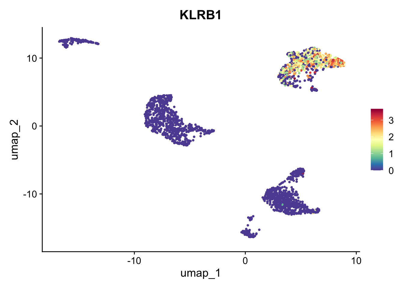
Paso 3. Guardar dataset
saveRDS(pbmc_annotated, file = "output/pbmc3k_singler_annotated.rds")Paso 4. Visualización de los datos
#visualizing the relative proportion of cell types across our samples
ggplot(pbmc_annotated[[]], aes(x = orig.ident, fill = immgen_singler_main)) +
  geom_bar(position = "fill") +
  scale_fill_viridis(discrete = TRUE)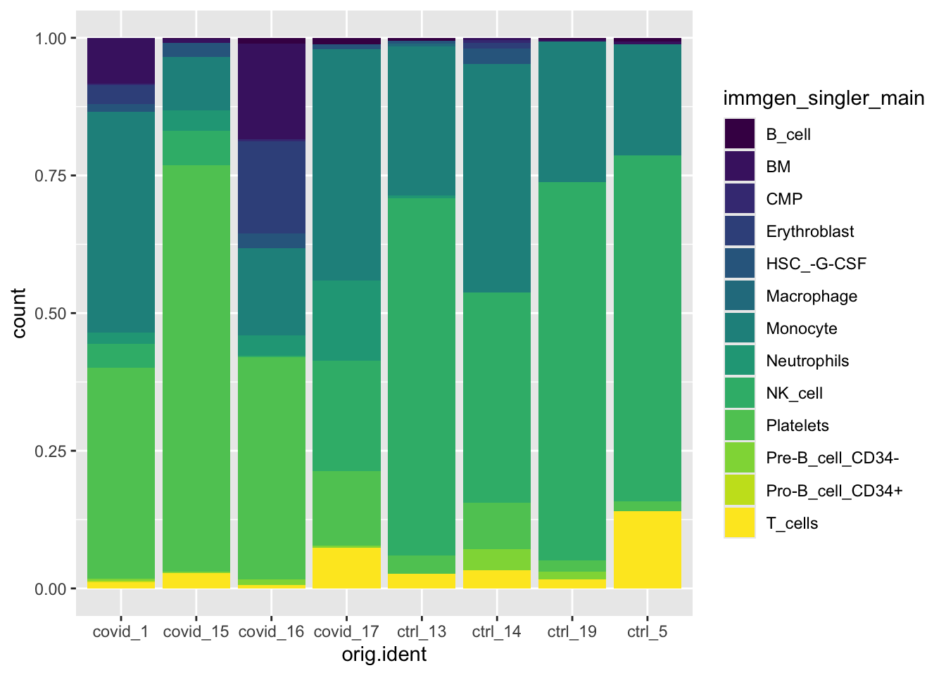
We can also flip the samples and cell labels and view this data as below.
ggplot(pbmc_annotated[[]], aes(x = immgen_singler_main, fill = orig.ident)) +
  geom_bar(position = "fill") +
  theme(axis.text.x = element_text(angle = 90, vjust = 0.5, hjust=1)) +
  scale_fill_viridis(discrete = TRUE)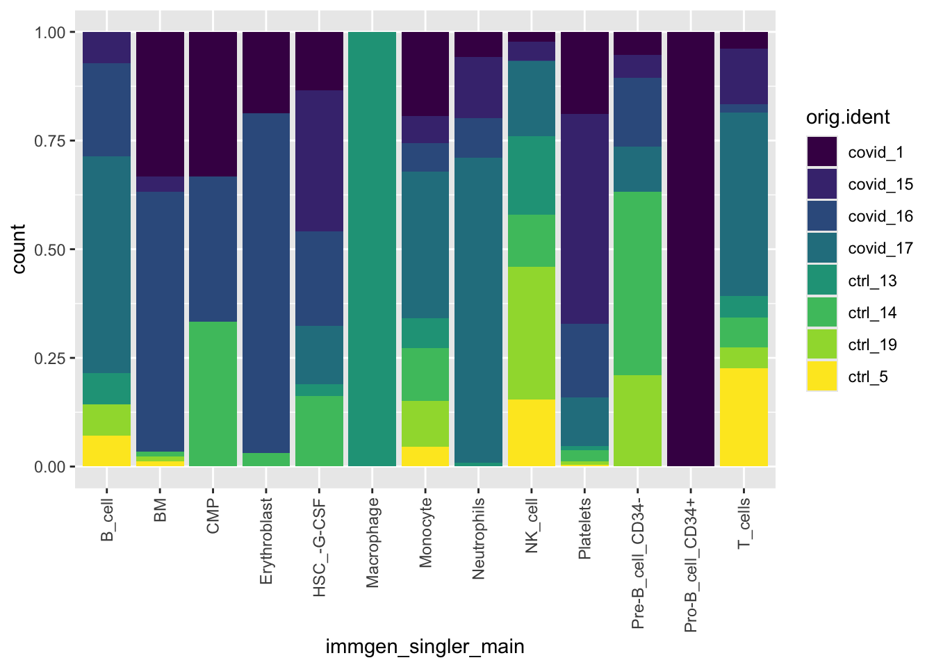
ggplot(pbmc_annotated[[]], aes(x = immgen_singler_fine, fill = orig.ident)) +
  geom_bar(position = "fill") +
  theme(axis.text.x = element_text(angle = 90, vjust = 0.5, hjust=1)) +
scale_fill_viridis(discrete = TRUE) 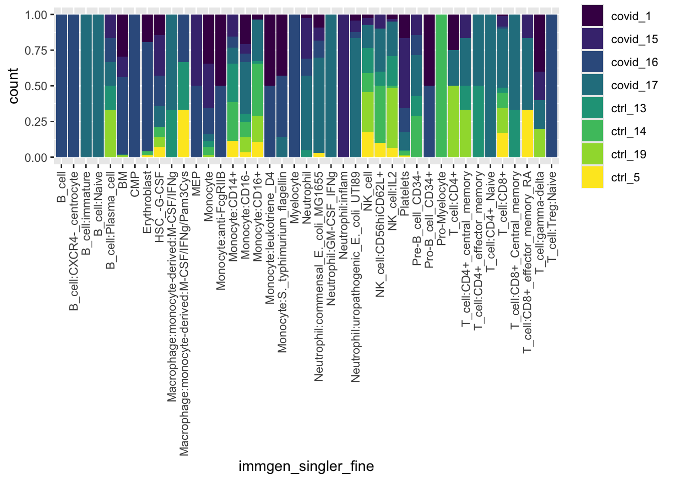
How do our cell type annotations map to our clusters we defined previously?
wrap_plots(
  # main
  DimPlot(pbmc_annotated, group.by = c("immgen_singler_main")) +
  # Eliminar axis
  NoAxes(),
  # fine
  DimPlot(pbmc_annotated, group.by = c("immgen_singler_fine")) +
  # Eliminar leyendas
  NoLegend() +
  # Eliminar axis
  NoAxes(),
ncol = 2)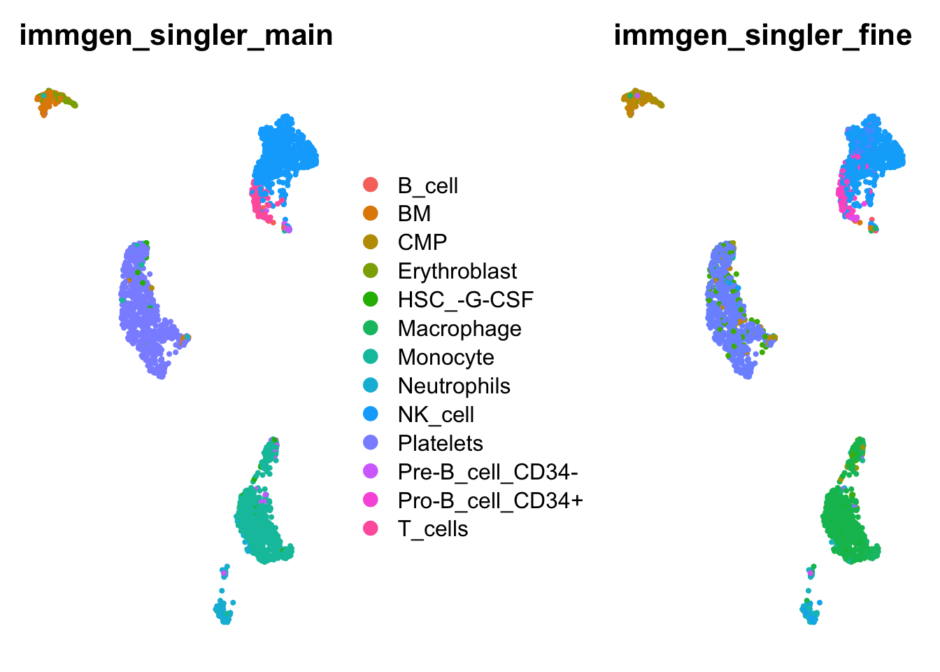
Si quieres separar y visualizar un tipo celular puedes
unique(pbmc_annotated$immgen_singler_main) [1] "Platelets" "CMP" "Monocyte" "BM"
[5] "Erythroblast" "Neutrophils" "NK_cell" "T_cells"
[9] "HSC_-G-CSF" "Pre-B_cell_CD34-" "Pro-B_cell_CD34+" "B_cell"
[13] "Macrophage" pbmc_annotated.celltype <- pbmc_annotated[, pbmc_annotated$immgen_singler_main == "Monocyte" ]
DimPlot(pbmc_annotated.celltype) +
# Eliminar leyendas
NoLegend() +
# Eliminar axis
NoAxes()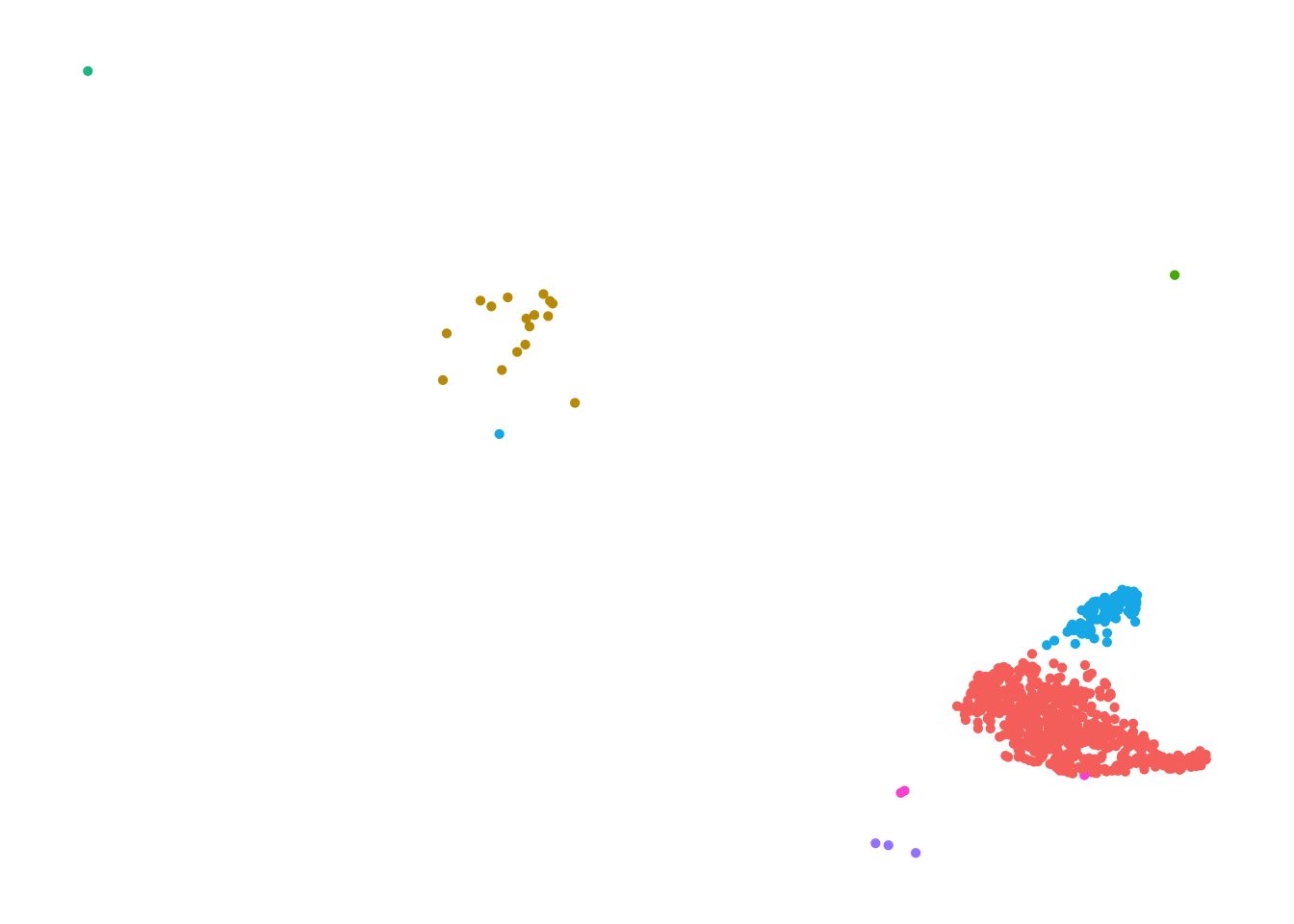
Paso 5. Ciclo celular
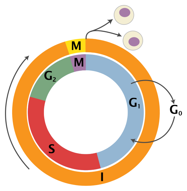
- Listas de genes de ciclo celular
- Seurat incluye listas de genes asociados a fase S y G2/M (
cc.genes.updated.2019).
- Asignar fases con
CellCycleScoring
# Cargar listas de genes
s.genes <- cc.genes.updated.2019$s.genes
g2m.genes <- cc.genes.updated.2019$g2m.genes

# Asignar ciclo celular
pbmc_annotated <- CellCycleScoring(pbmc_annotated,
                               s.features = s.genes,
                               g2m.features = g2m.genes,
                               set.ident = TRUE)

table(pbmc_annotated$orig.ident)
 covid_1 covid_15 covid_16 covid_17  ctrl_13  ctrl_14  ctrl_19   ctrl_5
     349      462      298      581      185      212      297      164
Esto añade columnas en meta.data con la fase asignada (Phase) y scores de S y G2M.
- Visualizar resultados
We can now create a violin plot for the cell cycle scores as well.
VlnPlot(pbmc_annotated, features = c("S.Score", "G2M.Score"), group.by = "orig.ident", ncol = 2, pt.size = .1)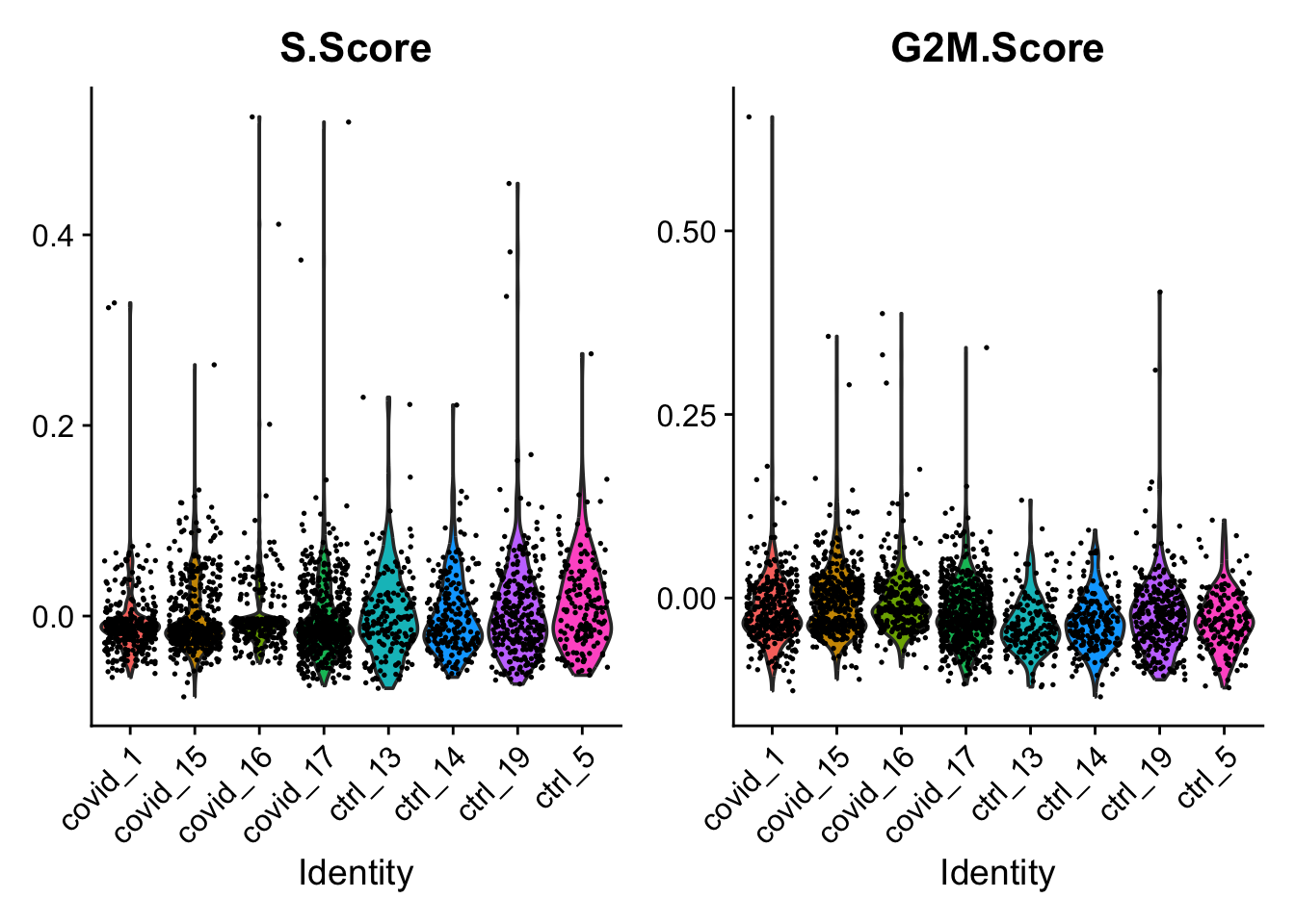
Finally, cell cycle score does not seem to depend on the cell type much - however, there are dramatic outliers in each group.
FeaturePlot(pbmc_annotated, features = c("S.Score","G2M.Score"),label.size = 4,repel = T,label = T) &
  theme(plot.title = element_text(size=10))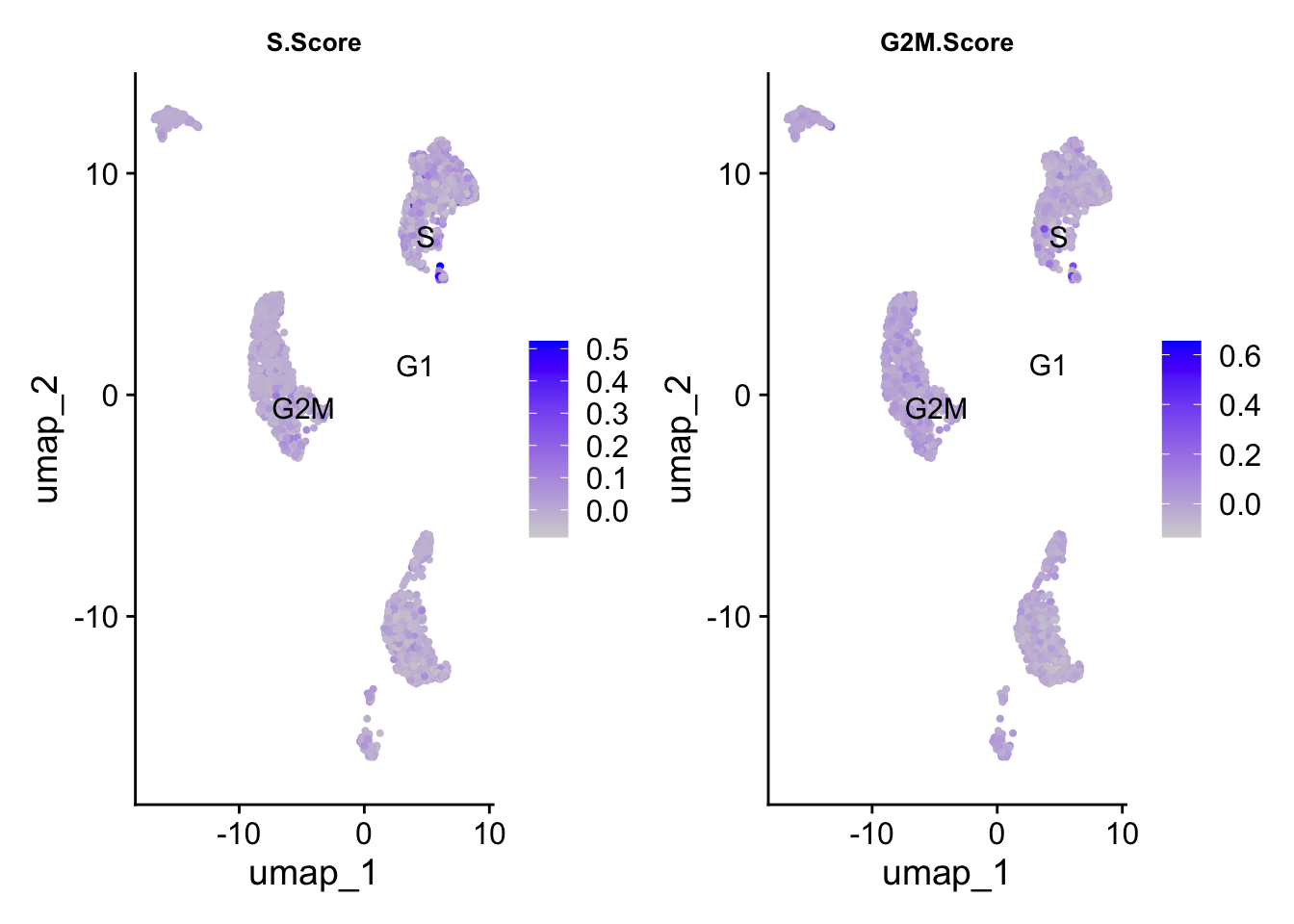
We can then check the cell phase on the UMAP. In this dataset, phase isn’t driving the clustering, and would not require any further handling.
DimPlot(pbmc_annotated, reduction = 'umap', group.by = "Phase")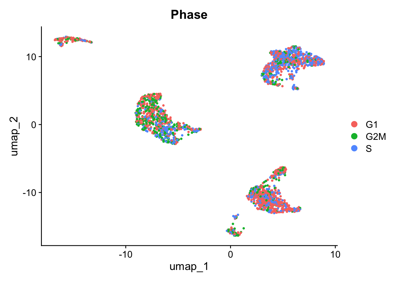
Where a bias is present, your course of action depends on the task at hand. It might involve ‘regressing out’ the cell cycle variation when scaling data ScaleData(kang, vars.to.regress="Phase"), omitting cell-cycle dominated clusters, or just accounting for it in your differential expression calculations.
If you are working with non-human data, you will need to convert these gene lists, or find new cell cycle associated genes in your species.
In this case it looks like we only have a few cycling cells in these datasets.
Seurat does an automatic prediction of cell cycle phase with a default cutoff of the scores at zero. As you can see this does not fit this data very well, so be cautious with using these predictions. Instead we suggest that you look at the scores.
FeatureScatter(pbmc_annotated, "S.Score", "G2M.Score", group.by = "Phase")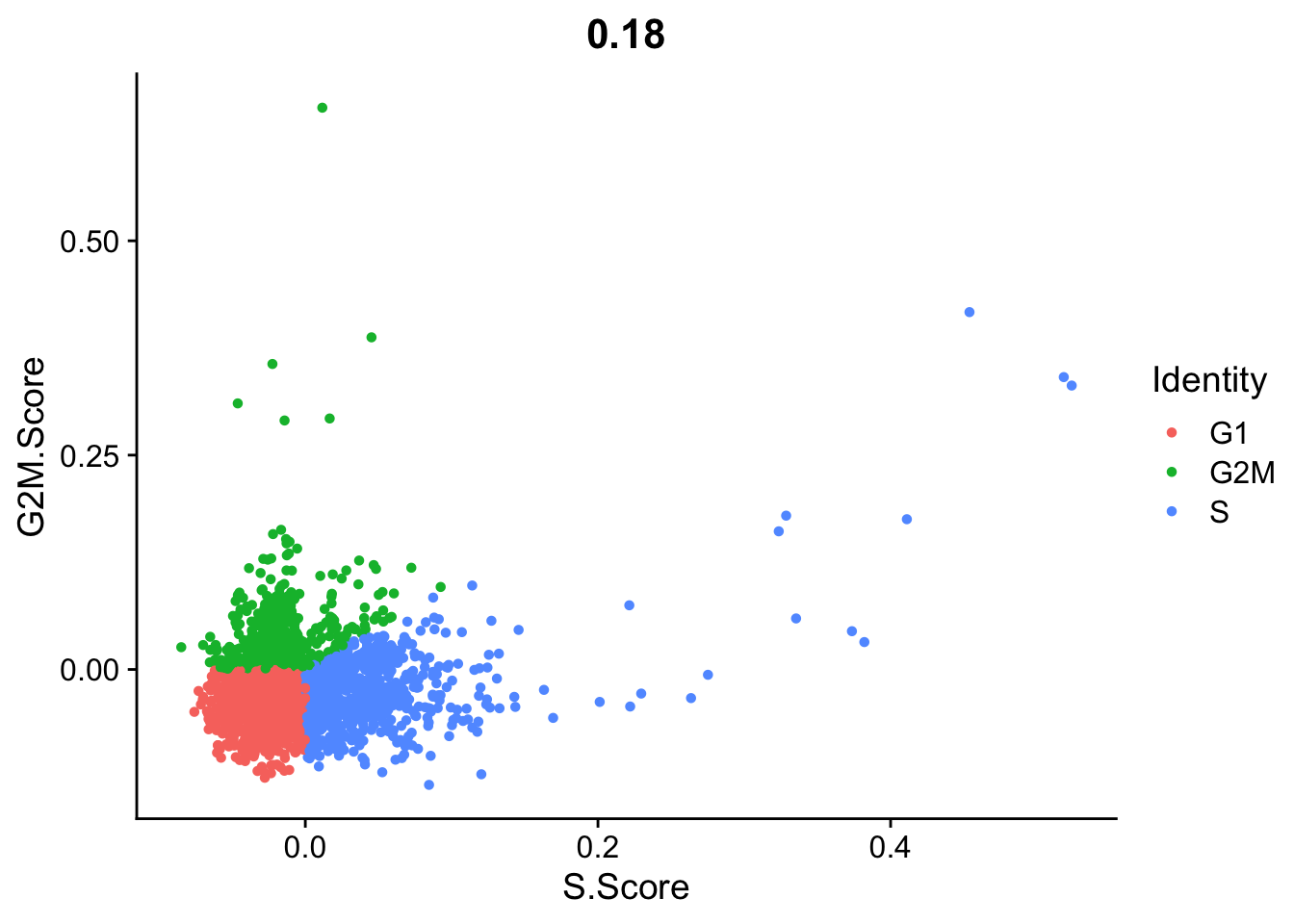
- Decidir si corregir
- Si el ciclo celular domina la variabilidad, se puede regredir en
ScaleData:
seurat_obj <- ScaleData(pbmc_annotated, vars.to.regress = c("S.Score", "G2M.Score"))Regressing out S.Score, G2M.ScoreCentering and scaling data matrixseurat_objAn object of class Seurat
33538 features across 2548 samples within 1 assay
Active assay: RNA (33538 features, 2000 variable features)
3 layers present: data, counts, scale.data
3 dimensional reductions calculated: pca, umap, harmony- Si es relevante biológicamente (ej. proliferación en tumores), se mantiene como variable de interés.
Paso 6. Expresión diferencial entre condiciones (type)
- Cambio de identidad
Estás definiendo que la identidad de las células (lo que Seurat usa para agrupar) sea la columna "type" del meta.data. Esto es importante porque FindAllMarkers usará esa identidad para comparar grupos.
sub_cell_selection <- alldata
sub_cell_selection <- SetIdent(sub_cell_selection, value = "type")- Análisis de Expresión diferencial (ctrl vs covid)
# Compute differentiall expression
DGE_cell_selection <- FindAllMarkers(sub_cell_selection,
    log2FC.threshold = 0.2,
    test.use = "wilcox",
    min.pct = 0.1,
    min.diff.pct = 0.2,
    only.pos = TRUE,
    max.cells.per.ident = 50,
    assay = "RNA"
)
Calculating cluster CovidCalculating cluster Ctrlhead(DGE_cell_selection) p_val avg_log2FC pct.1 pct.2 p_val_adj cluster gene
PF4 6.186534e-09 3.8520431 0.562 0.099 0.000207484 Covid PF4
CMTM5 3.854178e-07 3.6957634 0.389 0.047 0.012926141 Covid CMTM5
IGKC 4.828351e-07 0.5369594 0.430 0.049 0.016193322 Covid IGKC
CAVIN2 7.094952e-07 2.7348107 0.457 0.092 0.023795051 Covid CAVIN2
IFITM3 1.369915e-06 2.5344389 0.591 0.341 0.045944219 Covid IFITM3
CLEC1B 1.511224e-06 4.4492596 0.319 0.023 0.050683429 Covid CLEC1B- Análisis de Expresión diferencial (células del Cluster 3)
Si quiero ver la DEG en un solo cluster, por ejemplo en el Cluster 3:
# Supongamos que tu identidad actual es "seurat_clusters"
sub_cell_selection <- alldata
Idents(sub_cell_selection) <- "seurat_clusters"

# Comparar el cluster 3 contra todos los demás
DEG_cluster3 <- FindMarkers(sub_cell_selection,
    ident.1 = 3,
    log2FC.threshold = 0.25,
    test.use = "wilcox",
    min.pct = 0.1,
    min.diff.pct = 0.2,
    only.pos = TRUE
)

head(DEG_cluster3)
p_val avg_log2FC pct.1 pct.2 p_val_adj
TSC22D1 1.019876e-258 4.453454 0.917 0.131 3.420459e-254
HIST1H2BJ 3.876329e-242 4.257492 0.795 0.078 1.300043e-237
HIST1H3H 9.560991e-229 4.171782 0.835 0.112 3.206565e-224
ACRBP 2.537169e-217 3.583375 0.887 0.152 8.509159e-213
PTCRA 6.935459e-201 3.667611 0.786 0.109 2.326014e-196
HIST1H2AC 3.576061e-196 3.458317 0.963 0.268 1.199339e-191Paso 7. Visualización de Expresión diferencial entre condiciones (type)
We can now plot the expression across the type.
top5_cell_selection <- DGE_cell_selection %>%
    group_by(cluster) %>%
    top_n(-5, p_val)

VlnPlot(sub_cell_selection, features = as.character(unique(top5_cell_selection$gene)), ncol = 5, group.by = "type", assay = "RNA", pt.size = .1)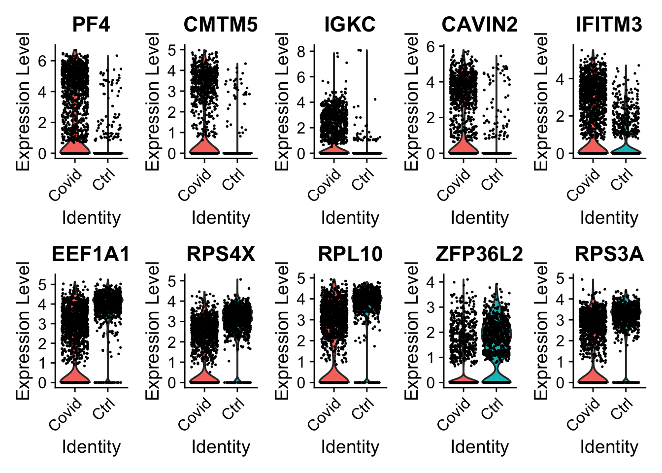
We can also plot these genes across all clusters, but split by type, to check if the genes are also over/under expressed in other celltypes.
VlnPlot(alldata,
    features = as.character(unique(top5_cell_selection$gene)),
    ncol = 4, split.by = "type", assay = "RNA", pt.size = 0
)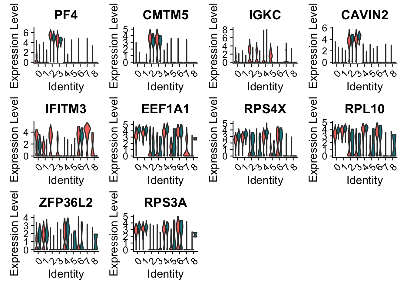
As you can see, we have many sex chromosome related genes among the top DE genes. And if you remember from the QC lab, we have unbalanced sex distribution among our subjects, so this may not be related to covid at all.
Paso 6. Pseudobulk (opcional)
cell_selection <- SetIdent(pbmc_annotated, value = "orig.ident")
table(cell_selection$orig.ident)
 covid_1 covid_15 covid_16 covid_17  ctrl_13  ctrl_14  ctrl_19   ctrl_5
     349      462      298      581      185      212      297      164
# get the count matrix for all cells
DGE_DATA <- GetAssayData(cell_selection, assay = "RNA", layer = "counts")
# Compute pseudobulk
mm <- Matrix::sparse.model.matrix(~ 0 + cell_selection$orig.ident)
pseudobulk <- DGE_DATA %*% mm# define the groups
bulk.labels <- c("Covid", "Covid", "Covid", "Covid", "Ctrl", "Ctrl", "Ctrl","Ctrl")
dge.list <- DGEList(counts = pseudobulk, group = factor(bulk.labels))
keep <- filterByExpr(dge.list)
dge.list <- dge.list[keep, , keep.lib.sizes = FALSE]
dge.list <- calcNormFactors(dge.list)
design <- model.matrix(~bulk.labels)
dge.list <- estimateDisp(dge.list, design)
fit <- glmQLFit(dge.list, design)
qlf <- glmQLFTest(fit, coef = 2)
topTags(qlf)Coefficient: bulk.labelsCtrl
logFC logCPM F PValue FDR
CDKN1A -2.673606 6.169782 90.64176 1.934901e-06 0.007689743
S100A12 -3.280002 10.406002 84.90719 2.573520e-06 0.007689743
BASP1 -2.804305 6.392202 75.85988 4.409343e-06 0.007689743
ASPH -2.813244 5.188133 73.27048 5.373808e-06 0.007689743
S100A8 -3.687406 14.320728 69.44833 6.506808e-06 0.007689743
SOD2 -2.493123 8.777729 67.51204 7.404662e-06 0.007689743
IGLC3 -6.597721 5.753170 47.69971 7.874225e-06 0.007689743
DSE -2.716279 5.603589 64.91069 9.162255e-06 0.007829147
PLBD1 -2.873686 8.054313 61.48260 1.131561e-05 0.008095002
MCEMP1 -3.431476 6.055396 60.77150 1.234736e-05 0.008095002As you can see, we have very few significant genes. Since we only have 4 vs 4 samples, we should not expect to find many genes with this method.
Again as dotplot including top 10 genes:
res.edgeR <- topTags(qlf, 100)$table
res.edgeR$dir <- ifelse(res.edgeR$logFC > 0, "Covid", "Ctrl")
res.edgeR$gene <- rownames(res.edgeR)

top.edgeR <- res.edgeR %>%
  group_by(dir) %>%
  top_n(-10, PValue) %>%
  arrange(dir)

DotPlot(cell_selection,
    features = as.character(unique(top.edgeR$gene)), group.by = "orig.ident",
    assay = "RNA"
) + coord_flip() + ggtitle("EdgeR pseudobulk") + RotatedAxis()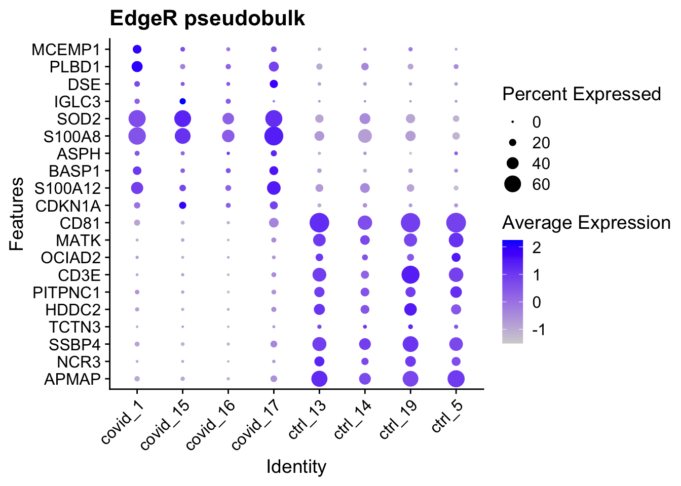
As you can see, even if we find few genes, they seem to make sense across all the patients.
Paso 9. Guardar dataset
save(dge.list, res.edgeR, cell_selection, file = "output/variables_expression.RData")Referencias
- Información del dataset de GEO GSE149689
- Más explicación de este dataset GSE149689
- SingleR + celldex + Seurat
- SingleR
- Differential gene expression
- Pseudobulk
- NBS - Celltype prediction
- Cell cycle Assignment
- Sanger - Cell type annotation using SingleR
- Differential Expression
- Análisis de expresión diferencial
- Introducción a Seurat
- Trajectory inference using Slingshot