4  scRNA‑seq — Errors & Survival

ImportantAbout Datasets

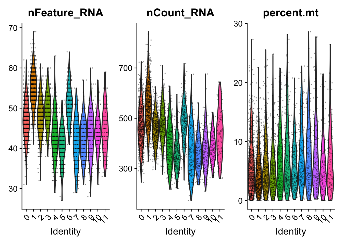
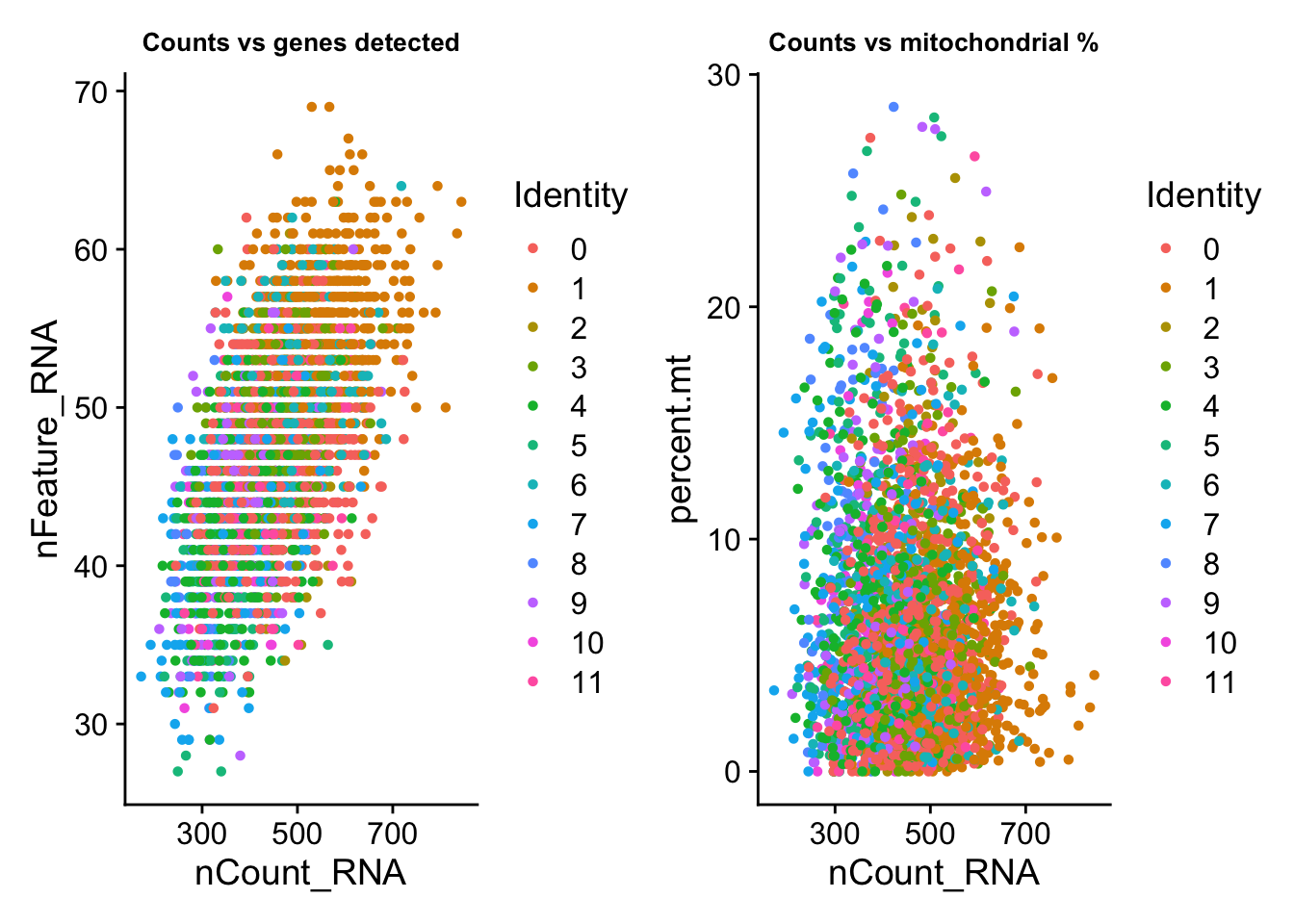
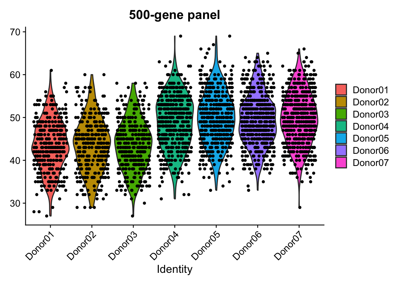
This dataset originates from GSE149689. The data have been reduced and deliberate errors were introduced for educational purposes.

Deliberate errors

Five steps were designed to fail (e.g., v4 slot access, incorrect use of GetAssayData slot=, wrong filter thresholds, dimensions greater than the number of principal components, plotting a label before adding it).

These steps are wrapped in try(), so the error prints to the console without halting the full run. The goal is for the user to read the error message, interpret it, and continue with the analysis.

4.1 Working Directory Options

When starting an analysis, you need to ensure that R knows where to find your scripts and data. There are two common approaches:

• Set Working Directory You can manually set the working directory in RStudio via: Session > Set Working Directory > To Source File Location. This option makes R run from the folder containing your script and the data/ subfolder. It is quick and useful for small or one-off scripts, but it requires resetting each time you open the project.

• Create an R Project The recommended approach for reproducibility and collaboration. An .Rproj file automatically sets the project root as the working directory. This allows you to use relative paths (e.g., data/file.csv) without manual adjustments. It also integrates seamlessly with Git/GitHub, Quarto, and RMarkdown, making your workflow more organized and consistent.

TipBest practice

For long-term projects, especially those shared on GitHub or used in teaching, creating an R Project is the most reliable option.

4.2 How to use

Run interactively, section by section (Ctrl+Enter / Cmd+Enter), from top to bottom. Do NOT source() the whole file in one go: several chunks are deliberate errors meant to be read, and Block 8 is optional take-home work that depends on a file released separately after the session.

4.3 Block 0 - Install packages and setup

4.3.1 Step 0.1 - Install packages

Checks each package before installing. If install.packages() fails, retries via BiocManager. Safe to run multiple times.

# Install BiocManager
if (!requireNamespace("BiocManager", quietly = TRUE))
  install.packages("BiocManager")

# All packages
all_pkgs <- c(
  "Seurat", "SeuratObject", "ggplot2", "patchwork",  "dplyr", "tidyr", "Matrix", "harmony", "scales", "ggrepel",
  "SingleR", "celldex", "BiocParallel", "scDblFinder",
  "SingleCellExperiment"
)

for (pkg in all_pkgs) {
  if (!requireNamespace(pkg, quietly = TRUE)) {
    message("Installing: ", pkg)
    tryCatch(install.packages(pkg, quiet = TRUE),
             error   = function(e) NULL,
             warning = function(w) NULL)
    if (!requireNamespace(pkg, quietly = TRUE)) {
      message("  CRAN failed. Retrying via BiocManager...")
      tryCatch(
        BiocManager::install(pkg, ask = FALSE, update = FALSE),
        error   = function(e) message("  FAILED: ", e$message),
        warning = function(w) NULL
      )
    }
    if (requireNamespace(pkg, quietly = TRUE))
      message("  OK: ", pkg, " (", as.character(packageVersion(pkg)), ")")
    else
      message("  FAILED: ", pkg, ". Run the fallback chunk below.")
  } else {
    message("Already installed: ", pkg,
            " (", as.character(packageVersion(pkg)), ")")
  }
}

Registered S3 method overwritten by 'data.table':
  method           from
  print.data.table     
Registered S3 method overwritten by 'htmlwidgets':
  method           from         
  print.htmlwidget tools:rstudio
Already installed: Seurat (5.5.0)
Already installed: SeuratObject (5.4.0)
Already installed: ggplot2 (4.0.3)
Already installed: patchwork (1.3.2)
Already installed: dplyr (1.2.1)
Already installed: tidyr (1.3.2)
Already installed: Matrix (1.7.5)
Already installed: harmony (2.0.4)
Already installed: scales (1.4.0)
Already installed: ggrepel (0.9.8)
Installing: SingleR
  CRAN failed. Retrying via BiocManager...
'getOption("repos")' replaces Bioconductor standard repositories, see
'help("repositories", package = "BiocManager")' for details.
Replacement repositories:
    CRAN: https://cran.rstudio.com/
Bioconductor version 3.23 (BiocManager 1.30.27), R 4.6.0 (2026-04-24)
Installing package(s) 'BiocVersion', 'SingleR'
also installing the dependencies ‘XVector’, ‘MatrixGenerics’, ‘GenomicRanges’, ‘Biobase’, ‘IRanges’, ‘Seqinfo’, ‘S4Arrays’, ‘SparseArray’, ‘SummarizedExperiment’, ‘BiocGenerics’, ‘S4Vectors’, ‘DelayedArray’, ‘beachmat’, ‘assorthead’

  FAILED: SingleR. Run the fallback chunk below.
Installing: celldex
  CRAN failed. Retrying via BiocManager...
'getOption("repos")' replaces Bioconductor standard repositories, see
'help("repositories", package = "BiocManager")' for details.
Replacement repositories:
    CRAN: https://cran.rstudio.com/
Bioconductor version 3.23 (BiocManager 1.30.27), R 4.6.0 (2026-04-24)
Installing package(s) 'BiocVersion', 'celldex'
also installing the dependencies ‘dir.expiry’, ‘dbplyr’, ‘Biostrings’, ‘XVector’, ‘rhdf5filters’, ‘V8’, ‘biocmake’, ‘h5mread’, ‘MatrixGenerics’, ‘GenomicRanges’, ‘Biobase’, ‘BiocGenerics’, ‘IRanges’, ‘Seqinfo’, ‘S4Arrays’, ‘BiocFileCache’, ‘BiocBaseUtils’, ‘KEGGREST’, ‘SparseArray’, ‘sparseMatrixStats’, ‘alabaster.schemas’, ‘rhdf5’, ‘jsonvalidate’, ‘assorthead’, ‘Rhdf5lib’, ‘HDF5Array’, ‘alabaster.ranges’, ‘blob’, ‘SummarizedExperiment’, ‘ExperimentHub’, ‘AnnotationHub’, ‘AnnotationDbi’, ‘S4Vectors’, ‘DelayedArray’, ‘DelayedMatrixStats’, ‘gypsum’, ‘alabaster.base’, ‘alabaster.matrix’, ‘alabaster.se’, ‘DBI’, ‘RSQLite’

  FAILED: celldex. Run the fallback chunk below.
Installing: BiocParallel
  CRAN failed. Retrying via BiocManager...
'getOption("repos")' replaces Bioconductor standard repositories, see
'help("repositories", package = "BiocManager")' for details.
Replacement repositories:
    CRAN: https://cran.rstudio.com/
Bioconductor version 3.23 (BiocManager 1.30.27), R 4.6.0 (2026-04-24)
Installing package(s) 'BiocVersion', 'BiocParallel'
also installing the dependencies ‘formatR’, ‘lambda.r’, ‘futile.options’, ‘futile.logger’, ‘snow’

  FAILED: BiocParallel. Run the fallback chunk below.
Installing: scDblFinder
  CRAN failed. Retrying via BiocManager...
'getOption("repos")' replaces Bioconductor standard repositories, see
'help("repositories", package = "BiocManager")' for details.
Replacement repositories:
    CRAN: https://cran.rstudio.com/
Bioconductor version 3.23 (BiocManager 1.30.27), R 4.6.0 (2026-04-24)
Installing package(s) 'BiocVersion', 'scDblFinder'
also installing the dependencies ‘formatR’, ‘lambda.r’, ‘futile.options’, ‘locfit’, ‘beeswarm’, ‘vipor’, ‘Cairo’, ‘cigarillo’, ‘RCurl’, ‘rjson’, ‘futile.logger’, ‘snow’, ‘assorthead’, ‘beachmat’, ‘ScaledMatrix’, ‘rsvd’, ‘MatrixGenerics’, ‘Biobase’, ‘Seqinfo’, ‘S4Arrays’, ‘edgeR’, ‘limma’, ‘statmod’, ‘metapod’, ‘SparseArray’, ‘ggbeeswarm’, ‘viridis’, ‘RcppML’, ‘pheatmap’, ‘ggrastr’, ‘UCSC.utils’, ‘Biostrings’, ‘XVector’, ‘Rhtslib’, ‘XML’, ‘GenomicAlignments’, ‘BiocIO’, ‘restfulr’, ‘SingleCellExperiment’, ‘BiocGenerics’, ‘BiocParallel’, ‘BiocNeighbors’, ‘BiocSingular’, ‘S4Vectors’, ‘SummarizedExperiment’, ‘scran’, ‘scater’, ‘scuttle’, ‘bluster’, ‘DelayedArray’, ‘xgboost’, ‘IRanges’, ‘GenomicRanges’, ‘GenomeInfoDb’, ‘Rsamtools’, ‘rtracklayer’

  FAILED: scDblFinder. Run the fallback chunk below.
Installing: SingleCellExperiment
  CRAN failed. Retrying via BiocManager...
'getOption("repos")' replaces Bioconductor standard repositories, see
'help("repositories", package = "BiocManager")' for details.
Replacement repositories:
    CRAN: https://cran.rstudio.com/
Bioconductor version 3.23 (BiocManager 1.30.27), R 4.6.0 (2026-04-24)
Installing package(s) 'BiocVersion', 'SingleCellExperiment'
also installing the dependencies ‘XVector’, ‘MatrixGenerics’, ‘Biobase’, ‘IRanges’, ‘Seqinfo’, ‘S4Arrays’, ‘SparseArray’, ‘SummarizedExperiment’, ‘S4Vectors’, ‘BiocGenerics’, ‘GenomicRanges’, ‘DelayedArray’

  FAILED: SingleCellExperiment. Run the fallback chunk below.

4.3.2 Step 0.2 - Verify and load all libraries

All packages are loaded here. No library() calls appear later in the script. If you see “namespace ggplot2 is imported by Seurat…” that is not an error; the package is already active. Always do Session > Restart R before opening the script.

pkgs <- c("Seurat", "SeuratObject", "ggplot2", "patchwork",
          "dplyr", "tidyr", "Matrix", "SingleR", "celldex",
          "harmony", "scales", "ggrepel", "BiocParallel",
          "scDblFinder", "SingleCellExperiment")

for (pkg in pkgs)
  cat(sprintf("  %-18s %s\n", pkg,
              ifelse(requireNamespace(pkg, quietly = TRUE), "OK", "MISSING")))

  Seurat             OK
  SeuratObject       OK
  ggplot2            OK
  patchwork          OK
  dplyr              OK
  tidyr              OK
  Matrix             OK
  SingleR            OK
  celldex            MISSING
  harmony            OK
  scales             OK
  ggrepel            OK
  BiocParallel       OK
  scDblFinder        OK
  SingleCellExperiment OK

cat("\nSeurat version:", as.character(packageVersion("Seurat")), "\n")

Seurat version: 5.5.1 

suppressPackageStartupMessages({
  library(Seurat);   library(SeuratObject); library(ggplot2)
  library(patchwork); library(dplyr);     library(tidyr);       library(Matrix)
  library(SingleR);  library(celldex);      library(BiocParallel)
  library(harmony);  library(scales);       library(ggrepel)
})

Warning: package 'Seurat' was built under R version 4.6.1

Error in `library()`:
! there is no package called 'celldex'

cat("\nAll libraries loaded.\n")

All libraries loaded.

Case 1: scDblFinder

The command used was:

BiocManager::install("scDblFinder", type="binary", dependencies=TRUE)

👉 In this case, the installation was successful because Bioconductor provides binary builds for macOS ARM64. By forcing type="binary", R avoided compiling C++ code, and all dependencies were installed without errors.

Case 2: celldex

The command was:

BiocManager::install("celldex", type="binary", dependencies=TRUE)

👉 Here the error persisted because one critical dependency (alabaster.base) does not yet have a binary build available. R attempted to compile it from source, but failed with the following error:

ld: library 'ssl' not found
clang++: error: linker command failed with exit code 1
ERROR: compilation failed for package ‘alabaster.base’
ERROR: dependency ‘alabaster.base’ is not available for package ‘celldex’

This means the compiler could not find the OpenSSL library required for linking. Even though we requested binary installation, Bioconductor has not yet published a binary for this dependency, so the error continues.

4.3.3 Step 0.3 - Folder structure and download files

Create and delete files

# Helper function to recreate a folder with messages
recreate_dir <- function(dir_name) {
  if (dir.exists(dir_name)) {
    cat(sprintf("The folder '%s' already exists. It will be deleted and recreated.\n", dir_name))
    unlink(dir_name, recursive = TRUE)  # delete folder and contents
  } else {
    cat(sprintf("The folder '%s' does not exist. It will be created.\n", dir_name))
  }
  dir.create(dir_name, showWarnings = FALSE)
}

# Apply the function to your folders
recreate_dir("data")

The folder 'data' already exists. It will be deleted and recreated.

recreate_dir("outputs")

The folder 'outputs' already exists. It will be deleted and recreated.

cat("Process completed. Folders are ready.\n")

Process completed. Folders are ready.

Download files

Here you will find the reduced files available for download from Google Drive.

FILE_ID <- "1mCg4VD91qK7pg-zL1iYUUBFWBr7fmmCM"
options(timeout = 600)
download.file(
  url      = paste0("https://drive.google.com/uc?export=download&confirm=t&id=",
                    FILE_ID),
  destfile = "data/gse149689_subset_3k.rds",
  mode     = "wb"
)
cat("File exists:", file.exists("data/gse149689_subset_3k.rds"), "\n")

File exists: TRUE 

cat("Size (MB)  :", round(file.size("data/gse149689_subset_3k.rds") / 1e6, 1), "\n")

Size (MB)  : 14.1 

4.3.4 Step 0.4 - reveal() helper (instructor use only)

Prints the answer + live-demo code for any QUESTION or PUZZLE in this script. Answers are NOT in this file. They live in a separate instructor_answers.R that only the instructor loads with source() before class. Students running reveal() in a fresh session see a brief notice and nothing else.

👉 Download: instructor_answers.R and reveal_function.R

#Instructor only
source("scripts/instructor_answers.R")

Instructor answers loaded. 47 entries. Try: reveal("1.2b")

source("scripts/reveal_function.R")

Usage:reveal("number")

reveal("5.2")

4.3.5 Step 0.5 - Namespace-safe accessor wrappers

In R, names that start with a dot (.) are usually used for internal helper functions. The function .safe_accessor is not meant to be called directly by the user. Instead, it builds the “safe” versions of Seurat’s accessor functions: SafeAssays, SafeLayers, and SafeReductions.

These safe wrappers make sure that the correct function is used even if different versions of Seurat or other Bioconductor packages introduce conflicts. Without them, you might get confusing errors when calling Assays(), Layers(), or Reductions() directly.

👉 Download: safe_accessor_function.R

Load it into your R session with:

#Instructor only
source("scripts/safe_accessor_function.R")

TipExplanation of Each Function

Use the safe functions in your analysis:

• SafeAssays(seurat_object)

  • Returns a list of all assays present in the Seurat object.
  • Safer than directly calling Assays() because it avoids issues if the object has unusual or corrupted assay slots.
  • Useful for checking what data types (RNA, ATAC, protein, etc.) are available before running downstream analysis.

SafeAssays(seurat_object)

• SafeLayers(seurat_object)

  • Lists all layers within a given assay (e.g., raw counts, normalized data, scaled data).
  • Helps you confirm which representations of the data are stored and prevents errors when switching between layers.
  • Important in multimodal workflows where multiple layers coexist.

SafeLayers(seurat_object)

• SafeReductions(seurat_object)

  • Shows all dimensionality reduction results (PCA, UMAP, t-SNE, etc.) stored in the object.
  • Ensures you know which reductions are available before plotting or clustering.
  • Prevents mistakes like calling DimPlot() on a reduction that doesn’t exist.

SafeReductions(seurat_object)

4.4 Block 1 - Object inspection (RNA + ADT)

Goal: Inspect the RNA assay, contrast it with the ADT assay, and walk through the layer system, the metadata, and the reductions slot.

4.4.1 Step 1.1 - Load the object

Loads the injected object (with embedded errors) when present, otherwise the clean object.

main_candidates <- c("data/gse149689_subset_3k_errors.rds",
                     "data/gse149689_subset_3k.rds")
main_path <- main_candidates[file.exists(main_candidates)][1]
if (is.na(main_path)) stop("No dataset found in data/. Expected one of: ",
                           paste(main_candidates, collapse = ", "))
sobj <- readRDS(main_path)
cat("Loaded:", main_path, "\n")

Loaded: data/gse149689_subset_3k.rds 

print(sobj)

An object of class Seurat 
524 features across 3000 samples within 2 assays 
Active assay: RNA (500 features, 500 variable features)
 3 layers present: counts, data, scale.data
 1 other assay present: ADT
 2 dimensional reductions calculated: pca, umap

TipQUESTION 1.1

• How many cells, how many features, how many assays?
• Which is the active (default) assay? Run the line below to get all four numbers.

cat("\nAnswer to QUESTION 1.1:\n")
cat("  Cells         :", ncol(sobj), "\n")
cat("  Features (RNA):", nrow(sobj[["RNA"]]), "\n")
cat("  Features (ADT):", nrow(sobj[["ADT"]]), "\n")
cat("  Assays        :", length(SafeAssays(sobj)), "(", paste(SafeAssays(sobj), collapse = ", "), ")\n")
cat("  Default assay :", DefaultAssay(sobj), "\n")

TipANSWER

3,000 cells across 2 assays. RNA assay has 500 features, a teaching-purpose subset (not the full transcriptome). ADT assay has 24 proteins. Default assay is RNA. The 500-gene subset matters: every QC threshold copied from a 33,000-gene tutorial will be wrong. This is the first opportunity to anchor the discussion of ‘tutorial defaults do not transfer’.

LIVE DEMO:

ncol(sobj)                    # cells

[1] 3000

nrow(sobj[["RNA"]])           # RNA features (500)

[1] 500

nrow(sobj[["ADT"]])           # ADT features (24)

[1] 24

Assays(sobj)                  # c("RNA", "ADT")

An object of class "SimpleAssays"
Slot "data":
List of length 1

DefaultAssay(sobj)            # "RNA"

[1] "RNA"

4.4.2 Step 1.1b - Add mitochondrial genes (this panel does not ship with any)

The 500-gene panel used for this course was curated around lineage and activation markers; it does not include MT- genes. Every QC step that depends on percent.mt ( Section 4.5, Block 2) needs a real signal to be useful, so we add 9 synthetic MT- genes here, with counts correlated to each cell’s total library size and a stress component for a subset of cells.

set.seed(7)
mt_gene_names <- c("MT-ND1", "MT-ND2", "MT-CO1", "MT-CO2", "MT-ATP8",
                    "MT-ATP6", "MT-CO3", "MT-ND3", "MT-CYB")

if (!any(grepl("^MT-", rownames(sobj[["RNA"]])))) {
  rna_counts  <- LayerData(sobj, assay = "RNA", layer = "counts")
  total_count <- Matrix::colSums(rna_counts)

  # A log-normal draw gives a continuous, right-skewed distribution: most
  # cells sit at a low, biologically typical fraction, with a gradual tail
  # toward the small subset of stressed/dying cells. This mirrors real PBMC
  # data, where percent.mt has no gap between "healthy" and "stressed"; it
  # is one continuous distribution that QC thresholds cut into at some
  # chosen point.
  n_cells     <- ncol(rna_counts)
  target_frac <- rlnorm(n_cells, meanlog = log(0.035), sdlog = 0.6)
  target_frac <- pmin(target_frac, 0.35)  # cap at a biologically plausible ceiling

  mt_total_per_cell <- round(total_count * target_frac)
  mt_total_per_cell[mt_total_per_cell < length(mt_gene_names)] <- length(mt_gene_names)

  # Spread each cell's MT total across the 9 genes with unequal weights
  # (mirrors real data, where MT-CO1/MT-CO3/MT-CYB are usually the highest).
  gene_weights <- c(0.10, 0.08, 0.22, 0.14, 0.03, 0.07, 0.18, 0.06, 0.12)
  mt_mat <- sapply(seq_len(n_cells), function(i) {
    as.integer(round(mt_total_per_cell[i] * gene_weights))
  })
  rownames(mt_mat) <- mt_gene_names
  colnames(mt_mat) <- colnames(rna_counts)
  mt_mat_sparse <- as(mt_mat, "CsparseMatrix")

  rna_counts_with_mt <- rbind(rna_counts, mt_mat_sparse)
  # The warning here ("Different cells and/or features from existing assay
  # RNA") comes from the [[<- replacement method noticing the new assay has
  # 509 features instead of 500, not from CreateAssay5Object itself. It is
  # the expected, harmless side effect of adding genes to an assay; wrap the
  # whole assignment so it does not look like an error in the console.
  new_rna_assay <- CreateAssay5Object(counts = rna_counts_with_mt)
  suppressWarnings(sobj[["RNA"]] <- new_rna_assay)
  DefaultAssay(sobj) <- "RNA"

  cat("Added", length(mt_gene_names), "synthetic MT- genes to the RNA assay.\n")
  cat("RNA assay now has", nrow(sobj[["RNA"]]), "features (was 500).\n")
} else {
  cat("MT- genes already present; skipping synthesis.\n")
}

MT- genes already present; skipping synthesis.

4.4.3 Step 1.2 - Seurat v4 vs v5: how the count matrix is stored

Seurat v5 changed how count matrices live inside an assay. v4 code that directly accesses @counts or uses slot= will error. The two patterns below are deliberate failures: read each error message.

# >>> DELIBERATE ERROR - read the message, then continue. <<<
try({
  # In Seurat v4, this was the standard way to get the count matrix.
  counts_old <- sobj@assays$RNA@counts
})

Error in try({ : 
  no slot of name "counts" for this object of class "Assay5"

# >>> DELIBERATE ERROR - read the message, then continue. <<<
try({
  counts_old2 <- GetAssayData(sobj, slot = "counts")
})

Error : The `slot` argument of `GetAssayData()` was deprecated in SeuratObject
5.0.0 and is now defunct.
ℹ Please use the `layer` argument instead.

TipExplanation

In Seurat v5, the @counts slot no longer exists in Assay5 objects. The correct argument is now layer = "counts". These errors are intentional examples: they show what happens when you run old pipeline scripts or receive objects created with older Seurat versions. Read the error message, understand why it occurs, and then continue.

Pattern 1: LayerData(). Recommended for Seurat v5.

counts_rna <- LayerData(sobj, assay = "RNA", layer = "counts")
cat("RNA counts matrix dimensions (genes x cells):\n")

RNA counts matrix dimensions (genes x cells):

cat(" ", dim(counts_rna), "\n\n")

  500 3000 

Pattern 1b: three equivalent ways to pull ONE gene’s counts without converting the whole sparse matrix to dense.

fetched <- FetchData(sobj, vars = "CD4", layer = "counts")[, 1]
indexed <- LayerData(sobj, assay = "RNA", layer = "counts")["CD4", ]
get_ad  <- GetAssayData(sobj, assay = "RNA", layer = "counts")["CD4", ]
cat("Three equivalent accessors for one gene's counts:\n")

Three equivalent accessors for one gene's counts:

cat("  FetchData            length:", length(fetched), " class:", class(fetched), "\n")

  FetchData            length: 3000  class: numeric 

cat("  LayerData[gene, ]    length:", length(indexed), " class:", class(indexed), "\n")

  LayerData[gene, ]    length: 3000  class: numeric 

cat("  GetAssayData[gene, ] length:", length(get_ad),  " class:", class(get_ad),  "\n")

  GetAssayData[gene, ] length: 3000  class: numeric 

cat("  All identical        :", all(fetched == indexed) && all(indexed == get_ad), "\n\n")

  All identical        : TRUE 

Pattern 2: assay class

cat("RNA assay class :", class(sobj[["RNA"]]), "\n")

RNA assay class : Assay5 

cat("ADT assay class :", class(sobj[["ADT"]]), "\n\n")

ADT assay class : Assay5 

Pattern 3: available layers

cat("RNA layers      :", paste(SafeLayers(sobj[["RNA"]]), collapse = ", "), "\n")

RNA layers      : counts, data, scale.data 

cat("ADT layers      :", paste(SafeLayers(sobj[["ADT"]]), collapse = ", "), "\n\n")

ADT layers      : counts, data 

Pattern 4: Seurat object version

cat("Object version  :", as.character(sobj@version), "\n")

Object version  : 5.1.0 

TipQUESTION 1.2

• What is the class of the RNA assay? And the ADT assay?
• Why might they be the same class even though the data behave very differently?

TipANSWER

Both are class Assay5. Assay5 is a storage container, not a normalization specification. The container holds a layer system (counts, data, scale.data) the same way for any modality. The differences between RNA and ADT (sparse vs dense, dropout vs bimodality, LogNormalize vs CLR, log scale vs CLR scale) are properties of the values stored in the layers and the chosen normalization, not of the assay class. A function operating on sobj[['ANY']] works mechanically on both. It also means running an RNA-specific normalization on ADT does not throw a type error.

LIVE DEMO:

class(sobj[["RNA"]])    # "Assay5"

[1] "Assay5"
attr(,"package")
[1] "SeuratObject"

class(sobj[["ADT"]])    # "Assay5"

[1] "Assay5"
attr(,"package")
[1] "SeuratObject"

# Same class, different content. Confirm by inspecting layers:
Layers(sobj[["RNA"]])   # counts (data and scale.data appear after preprocessing)

[1] "counts"     "data"       "scale.data"

Layers(sobj[["ADT"]])   # counts

[1] "counts" "data"  

TipQUESTION 1.2c

FetchData(), LayerData()[gene, ], and GetAssayData()[gene, ] are all equivalent here. Why might they NOT be equivalent for normalized data instead of raw counts? (Think about what each function defaults to for the layer argument).

TipANSWER

On the counts layer all three read raw integer values from the same underlying sparse matrix, so the result is identical. For normalized data they differ in argument defaults: FetchData() defaults to layer='data' (normalized); LayerData() takes layer= explicitly; GetAssayData() in newer Seurat also expects layer= (slot= is deprecated, see E2). Mismatches appear when one call defaults to data and another to counts. Always pass layer= explicitly.

LIVE DEMO:

# After Block 4:
fd <- FetchData(sobj_filt, vars = "CD3E")[, 1] # data layer
lc <- LayerData(sobj_filt, assay="RNA", layer="counts")["CD3E", ] # counts
ld <- LayerData(sobj_filt, assay="RNA", layer="data")["CD3E", ] # data
all(fd == ld)   # TRUE
all(fd == lc)   # FALSE (different layers)

4.4.4 Step 1.2b - Full slot map of a Seurat object

A Seurat object has more slots than most tutorials show. Some hold raw data, some hold derived results, some are caches, some are metadata about the analysis history. The same value often lives in two or three places by design. Knowing the map prevents three classes of bug:

1. Reading from the wrong copy after one is updated.
2. Failing to find data that exists under a slot you did not know.
3. Trusting downstream results when an upstream slot was overwritten.

A.1 - Top-level slots: print every slot name and a 1-line description of each

cat("\n== TOP-LEVEL SLOTS ==\n")

== TOP-LEVEL SLOTS ==

top_slots <- slotNames(sobj)
for (s in top_slots) cat(sprintf("  @%-15s class: %s\n", s, class(slot(sobj, s))[1]))

  @assays          class: list
  @meta.data       class: data.frame
  @active.assay    class: character
  @active.ident    class: factor
  @graphs          class: list
  @neighbors       class: list
  @reductions      class: list
  @images          class: list
  @project.name    class: character
  @misc            class: list
  @version         class: package_version
  @commands        class: list
  @tools           class: list

A.2 - @assays: list of assays. Each assay is an Assay5 (v5) or Assay (v4)

cat("\n== @assays ==\n")

== @assays ==

cat("  Assay names              :", paste(names(sobj@assays), collapse = ", "), "\n")

  Assay names              : RNA, ADT 

cat("  Active assay             :", DefaultAssay(sobj), "\n")

  Active assay             : RNA 

cat("  Number of assays         :", length(sobj@assays), "\n")

  Number of assays         : 2 

Inside one assay (v5 Assay5), the slot map is different from v4:

cat("\n  [inside sobj[['RNA']] (v5 Assay5)]\n")

  [inside sobj[['RNA']] (v5 Assay5)]

rna_assay_slots <- slotNames(sobj[["RNA"]])
for (s in rna_assay_slots) {
  val <- slot(sobj[["RNA"]], s)
  cat(sprintf("    @%-15s class: %-15s length/dim: %s\n",
              s, class(val)[1],
              if (is.list(val))    paste0("list of ", length(val))
              else if (is.null(dim(val))) paste0("len ", length(val))
              else paste(dim(val), collapse = " x ")))
}

    @layers          class: list            length/dim: list of 3
    @cells           class: LogMap          length/dim: 3000 x 3
    @features        class: LogMap          length/dim: 500 x 3
    @default         class: integer         length/dim: len 1
    @assay.orig      class: character       length/dim: len 0
    @meta.data       class: data.frame      length/dim: list of 8
    @misc            class: list            length/dim: list of 0
    @key             class: character       length/dim: len 1

A.3 - @meta.data: cell-level metadata data.frame

Rows = cells. Columns` = whatever was added during preprocessing.

cat("\n== @meta.data (cell-level) ==\n")

== @meta.data (cell-level) ==

cat("  Dimensions       :", dim(sobj@meta.data)[1], "cells x",
                            dim(sobj@meta.data)[2], "columns\n")

  Dimensions       : 3000 cells x 14 columns

cat("  Column names     :\n")

  Column names     :

print(colnames(sobj@meta.data))

 [1] "orig.ident"      "nCount_RNA"      "nFeature_RNA"    "percent.mt"     
 [5] "donor_id"        "condition"       "severity"        "age"            
 [9] "cell_type"       "nCount_ADT"      "nFeature_ADT"    "percent.ribo"   
[13] "RNA_snn_res.0.5" "seurat_clusters"

A.4 - @active.ident: a FACTOR over cells. The current "identity" used by downstream Seurat functions (FindMarkers, DimPlot group.by = NULL default)

It is independent of the metadata columns and is set by SetIdent / Idents().

cat("\n== @active.ident ==\n")

== @active.ident ==

cat("  Class            :", class(sobj@active.ident), "\n")

  Class            : factor 

cat("  Levels currently :", paste(head(levels(sobj@active.ident), 5), collapse = ", "),
                             ifelse(length(levels(sobj@active.ident)) > 5, " ...", ""), "\n")

  Levels currently : 0, 1, 2, 3, 4  ... 

cat("  First 5 cells    :\n")

  First 5 cells    :

print(head(sobj@active.ident, 5))

CELL000001 CELL000011 CELL000021 CELL000031 CELL000041 
         8          9         10          5          2 
Levels: 0 1 2 3 4 5 6 7 8 9 10 11

A.5 - @reductions: list of DimReduc objects (pca, umap, harmony, etc.)

Each one has its OWN slots: cell.embeddings (cells x dims), feature.loadings (features x dims), stdev (per-dim variance), key (column prefix), assay.used.

cat("\n== @reductions ==\n")

== @reductions ==

cat("  Reductions present:", paste(names(sobj@reductions), collapse = ", "), "\n")

  Reductions present: pca, umap 

if (length(sobj@reductions) > 0) {
  for (red_name in names(sobj@reductions)) {
    red <- sobj@reductions[[red_name]]
    cat(sprintf("  [%s]\n", red_name))
    cat(sprintf("    cell.embeddings : %s\n", paste(dim(red@cell.embeddings), collapse = " x ")))
    cat(sprintf("    feature.loadings: %s\n", paste(dim(red@feature.loadings), collapse = " x ")))
    cat(sprintf("    stdev length    : %d\n", length(red@stdev)))
    cat(sprintf("    key             : %s\n", red@key))
    cat(sprintf("    assay.used      : %s\n", red@assay.used))
  }
} else {
  cat("  (none yet; PCA/UMAP happen in Block 4)\n")
}

  [pca]
    cell.embeddings : 3000 x 30
    feature.loadings: 500 x 30
    stdev length    : 30
    key             : PC_
    assay.used      : RNA
  [umap]
    cell.embeddings : 3000 x 2
    feature.loadings: 0 x 0
    stdev length    : 0
    key             : umap_
    assay.used      : RNA

A.6 - @graphs and @neighbors: caches filled by FindNeighbors. Empty here

cat("\n== @graphs and @neighbors ==\n")

== @graphs and @neighbors ==

cat("  Graphs    :", ifelse(length(sobj@graphs)    == 0, "empty (filled by FindNeighbors)",
                            paste(names(sobj@graphs), collapse = ", ")), "\n")

  Graphs    : RNA_nn, RNA_snn 

cat("  Neighbors :", ifelse(length(sobj@neighbors) == 0, "empty (filled by FindNeighbors)",
                            paste(names(sobj@neighbors), collapse = ", ")), "\n")

  Neighbors : empty (filled by FindNeighbors) 

A.7 - @commands: every Seurat function call ever made on this object, with all arguments, providing a full analysis history. If you ever wonder “what arguments did the previous user pass to NormalizeData?”, check here.

cat("\n== @commands (analysis history) ==\n")

== @commands (analysis history) ==

cat("  Commands recorded:", length(sobj@commands), "\n")

  Commands recorded: 8 

if (length(sobj@commands) > 0) {
  cat("  First 5 command names:\n")
  print(head(names(sobj@commands), 5))
  # Inspect one command in detail
  first_cmd <- sobj@commands[[1]]
  cat(sprintf("\n  [detail of first command: %s]\n", names(sobj@commands)[1]))
  cat("    call.string   :", first_cmd@call.string[1], "\n")
  cat("    time.stamp    :", as.character(first_cmd@time.stamp), "\n")
  cat("    assay.used    :", first_cmd@assay.used, "\n")
  cat("    params (names):", paste(names(first_cmd@params), collapse = ", "), "\n")
}

  First 5 command names:
[1] "NormalizeData.RNA"        "FindVariableFeatures.RNA"
[3] "ScaleData.RNA"            "RunPCA.RNA"              
[5] "FindNeighbors.RNA.pca"   

  [detail of first command: NormalizeData.RNA]
    call.string   : NormalizeData(sobj, verbose = FALSE) 
    time.stamp    : 2026-05-19 18:41:26.947809 
    assay.used    : RNA 
    params (names): assay, normalization.method, scale.factor, margin, verbose 

A.8 - @misc, @tools, @project.name, @version: small administrative slots

cat("\n== Administrative slots ==\n")

== Administrative slots ==

cat("  @project.name :", sobj@project.name, "\n")

  @project.name : GSE149689 

cat("  @version      :", as.character(sobj@version), "\n")

  @version      : 5.1.0 

cat("  @misc names   :", ifelse(length(sobj@misc) == 0, "empty",
                                paste(names(sobj@misc), collapse = ", ")), "\n")

  @misc names   : empty 

cat("  @tools names  :", ifelse(length(sobj@tools) == 0, "empty",
                                paste(names(sobj@tools), collapse = ", ")), "\n")

  @tools names  : empty 

A.9 - Same data, different paths: a common source of confusion.

The values below are IDENTICAL, but accessed through different slots/accessors.

cat("\n== Same data, different paths (sanity proofs) ==\n")

== Same data, different paths (sanity proofs) ==

cat("Test 1: assay access\n")

Test 1: assay access

cat("  identical(sobj@assays$RNA, sobj[['RNA']])           :",
    identical(sobj@assays$RNA, sobj[["RNA"]]), "\n")

  identical(sobj@assays$RNA, sobj[['RNA']])           : TRUE 

cat("Test 2: metadata column access (4 equivalent paths)\n")

Test 2: metadata column access (4 equivalent paths)

v1 <- sobj$nFeature_RNA
v2 <- sobj@meta.data$nFeature_RNA
v3 <- sobj[[]]$nFeature_RNA
v4 <- FetchData(sobj, vars = "nFeature_RNA")[, 1]

identical() is sensitive to attributes (names, integer vs numeric storage) that differ across these four accessors even when every value is the same.

Strip names and coerce type before comparing, since the point here is value equality, not attribute equality.

all_match <- all(unname(as.numeric(v1)) == unname(as.numeric(v2))) &&
             all(unname(as.numeric(v2)) == unname(as.numeric(v3))) &&
             all(unname(as.numeric(v3)) == unname(as.numeric(v4)))
cat("  all four return the same values                     :", all_match, "\n")

  all four return the same values                     : TRUE 

cat("  (identical() can still report FALSE here; that compares attributes\n")

  (identical() can still report FALSE here; that compares attributes

cat("   like names or integer-vs-numeric storage, not the values themselves)\n")

   like names or integer-vs-numeric storage, not the values themselves)

cat("Test 3: cell name access (3 equivalent paths)\n")

Test 3: cell name access (3 equivalent paths)

cat("  identical(Cells(sobj), colnames(sobj))              :",
    identical(Cells(sobj), colnames(sobj)), "\n")

  identical(Cells(sobj), colnames(sobj))              : TRUE 

cat("  identical(Cells(sobj), rownames(sobj@meta.data))    :",
    identical(Cells(sobj), rownames(sobj@meta.data)), "\n")

  identical(Cells(sobj), rownames(sobj@meta.data))    : TRUE 

cat("Test 4: feature name access (varies with default assay)\n")

Test 4: feature name access (varies with default assay)

cat("  rownames(sobj) returns features of the ACTIVE assay only\n")

  rownames(sobj) returns features of the ACTIVE assay only

cat("  default assay is", DefaultAssay(sobj), "\n")

  default assay is RNA 

cat("  identical(rownames(sobj), Features(sobj))           :",
    identical(rownames(sobj), Features(sobj)), "\n")

  identical(rownames(sobj), Features(sobj))           : TRUE 

cat("  identical(rownames(sobj), rownames(sobj[['RNA']])) :",
    identical(rownames(sobj), rownames(sobj[["RNA"]])), "\n")

  identical(rownames(sobj), rownames(sobj[['RNA']])) : TRUE 

cat("  identical(rownames(sobj), rownames(sobj[['ADT']])) :",
    identical(rownames(sobj), rownames(sobj[["ADT"]])), "\n")

  identical(rownames(sobj), rownames(sobj[['ADT']])) : FALSE 

cat("  >> rownames depends on DefaultAssay. Always pass assay= explicitly.\n")

  >> rownames depends on DefaultAssay. Always pass assay= explicitly.

A.10 - SLOT PUZZLES: where would you look to find each item below?

Try to write the answer in your head before running.

cat("\n== SLOT PUZZLES (try before running) ==\n")

== SLOT PUZZLES (try before running) ==

TipPUZZLE 1.2b/1

Where is the original Seurat version that created this object?

cat("\nPUZZLE 1: original Seurat version that created this object?\n")

PUZZLE 1: original Seurat version that created this object?

cat("  Answer: sobj@version (top-level slot)\n")

  Answer: sobj@version (top-level slot)

cat("  Value :", as.character(sobj@version), "\n")

  Value : 5.1.0 

TipANSWER

sobj@version. Top-level slot that records the Seurat version that originally constructed the object, not the version currently loaded. Useful when debugging v4-to-v5 migration issues.

LIVE DEMO:

sobj@version

[1] '5.1.0'

packageVersion("Seurat")   # version currently loaded

[1] '5.5.1'

TipQUESTION 1.2b

For each of the 4 sanity-proof tests above (A.9), which one is GUARANTEED to be identical regardless of analysis state, and which one DEPENDS on DefaultAssay? Why is the distinction important when sharing code?

TipANSWER

Tests 1 and 3 are guaranteed identical via identical(): assay access (sobj[['RNA']] vs sobj@assays$RNA) always returns the same Assay5 object, and cell names always live in colnames(sobj). Test 2 (metadata column access) is more subtle than it looks: sobj$nFeature_RNA, sobj@meta.data$nFeature_RNA, and sobj[[]]$nFeature_RNA return the same named vector, but FetchData(sobj, vars='nFeature_RNA')[, 1] drops the cell-name attribute when the data.frame column is extracted with [, 1]. The VALUES are identical; identical() is not, because it also compares the names attribute. This is a good example of identical() being too strict for the question actually being asked: when verifying value equality across accessors, strip names (e.g. unname()) or compare numerically (all(x == y)) instead of using identical() directly. Test 4 is the trap with real consequences: rownames(sobj) returns features of the ACTIVE assay only. If a collaborator writes marker %in% rownames(sobj) assuming RNA, but the active assay has been set to ADT, the check fails silently for any gene that is not also a protein name. General rule when sharing or receiving code: pass assay= explicitly whenever a function call could resolve differently depending on the active assay, and do not assume identical() failing means the values differ; it can also mean only an attribute differs.

LIVE DEMO:

# Run the 4 tests live:
identical(sobj@assays$RNA, sobj[["RNA"]])                  # TRUE always

[1] TRUE

# Test 2: identical() can be FALSE here even though values match,
# because FetchData()[, 1] drops cell names that $ and [[]] keep:
identical(sobj$nFeature_RNA, sobj@meta.data$nFeature_RNA)  # TRUE

[1] FALSE

v4 <- FetchData(sobj, vars = "nFeature_RNA")[, 1]
identical(sobj$nFeature_RNA, v4)                           # often FALSE (names)

[1] FALSE

all(unname(sobj$nFeature_RNA) == unname(v4))               # TRUE (values match)

[1] TRUE

identical(Cells(sobj), colnames(sobj))                     # TRUE always

[1] TRUE

# Now the trap:
DefaultAssay(sobj) <- "RNA"; head(rownames(sobj))          # gene symbols

[1] "CD3E" "CD3D" "CD3G" "CD4"  "CD8A" "CD8B"

DefaultAssay(sobj) <- "ADT"; head(rownames(sobj))          # protein names (different)

[1] "CD3"  "CD4"  "CD8a" "CD14" "CD16" "CD19"

DefaultAssay(sobj) <- "RNA"                                # restore

4.4.5 Step 1.3 - Inspecting the RNA assay (intermediate)

Three properties of a single-cell RNA count matrix that drive every later decision: sparsity, memory footprint, and layer state. Inspect them now, before any normalization or scaling. The ADT counterpart to this step opens Block 6 (Section 5.1), once the CITE-seq workflow actually needs it.

Sparsity = fraction of zero entries. Drives normalization decisions.

counts_mat <- LayerData(sobj, assay = "RNA", layer = "counts")
total_entries  <- prod(dim(counts_mat))
nonzero        <- Matrix::nnzero(counts_mat)
sparsity       <- 1 - nonzero / total_entries

cat("RNA count matrix:\n")

RNA count matrix:

cat("  Genes   :", nrow(counts_mat), "\n")

  Genes   : 500 

cat("  Cells   :", ncol(counts_mat), "\n")

  Cells   : 3000 

cat("  Total entries  :", format(total_entries, big.mark = ","), "\n")

  Total entries  : 1,500,000 

cat("  Non-zero entries:", format(nonzero, big.mark = ","), "\n")

  Non-zero entries: 142,375 

cat("  Sparsity        :", round(sparsity * 100, 1), "%\n\n")

  Sparsity        : 90.5 %

TipQUESTION 1.3a

A typical full-transcriptome PBMC dataset shows RNA sparsity above 90%. This 500+9-gene panel is lower. What does the sparsity value you just printed tell you about gene panel size versus dropout rate?

TipANSWER

Sparsity in this panel is lower than a full transcriptome mainly because the 500 genes were curated to be lineage and activation markers, which tend to be more highly and consistently expressed than the average gene in a full transcriptome (most genes in a full panel are low-expressed or cell-type-restricted, which is what drives sparsity above 90%). A smaller, curated panel is not immune to dropout: the same capture and reverse-transcription inefficiencies apply per molecule regardless of panel size. What changes is the average expression level of the genes included, not the underlying biology of dropout. This distinction matters when reading a sparsity number from any dataset: a low sparsity value can mean a curated panel of well-expressed genes, not necessarily a technically superior experiment.

LIVE DEMO:

rna <- LayerData(sobj, assay="RNA", layer="counts")
mean(rna == 0) * 100        # RNA sparsity % for this panel

[1] 90.50833

Compare to a full-transcriptome expectation (commonly 90%+ for 10x PBMC)

CautionCaution

Dense vs sparse storage matters at scale. A full 10x experiment with 50,000 cells and 33,000 genes as a dense matrix exceeds 50 GB.

4.4.6 Compare sparse (counts) vs dense (after scaling) memory

counts_rna_sz <- object.size(LayerData(sobj, assay = "RNA", layer = "counts"))
cat("RNA counts layer (sparse):", format(counts_rna_sz, units = "Mb"), "\n")

RNA counts layer (sparse): 1.9 Mb 

The full object:

obj_size <- object.size(sobj)
cat("Full Seurat object       :", format(obj_size, units = "Mb"), "\n\n")

Full Seurat object       : 23.9 Mb 

cat("\nscale.data is a DENSE genes-by-cells matrix.\n")

scale.data is a DENSE genes-by-cells matrix.

cat("On full datasets, scale only the genes used in PCA to keep memory bounded.\n")

On full datasets, scale only the genes used in PCA to keep memory bounded.

TipQUESTION 1.3b

The counts layer is sparse, the scale.data layer is dense. Project this to a 50,000-cell, 33,000-gene experiment: what is the memory implication, and what does it tell you about how to use ScaleData?

TipANSWER

Dense double matrix: 33,000 features x 50,000 cells x 8 bytes = 13.2 GB. A sparse representation at 90% sparsity stores about 33,000 x 50,000 x 0.10 nonzeros x 16 bytes per nonzero = 2.6 GB. ScaleData centers and scales each feature, producing a dense matrix even when input was sparse. Running ScaleData on all features at this scale will exhaust RAM on any laptop. Standard practice: scale only the highly variable genes used in PCA, typically 2,000-3,000 features. The dense scaled matrix becomes 3,000 x 50,000 x 8 = 1.2 GB, manageable. Pass features = VariableFeatures(sobj) to ScaleData.

LIVE DEMO:

object.size(LayerData(sobj, assay="RNA", layer="counts"))   # sparse

1973416 bytes

object.size(as.matrix(LayerData(sobj, assay="RNA", layer="counts")))  # dense

12251800 bytes

Best practice (already used in Step 4.4, Section 4.7.4):

ScaleData(sobj, features = VariableFeatures(sobj))

4.4.7 Step 1.6 - Metadata

Reductions (PCA, UMAP, Harmony, etc.) are computed in Block 4 (Section 4.7) onward. At this point in the script, none exist yet. Confirm that explicitly instead of assuming it: it is the same habit as checking DefaultAssay() before trusting any accessor. The access patterns for cell.embeddings and feature.loadings are covered in Step 4.4, (Section 4.7.4), once PCA actually exists.

cat("Reductions in the object:\n")

Reductions in the object:

print(SafeReductions(sobj))

[1] "pca"  "umap"

cat("(empty; PCA happens in Block 4.)\n\n")

(empty; PCA happens in Block 4.)

cat("Metadata columns and types:\n")

Metadata columns and types:

str(sobj@meta.data)

'data.frame':   3000 obs. of  14 variables:
 $ orig.ident     : chr  "Donor01" "Donor01" "Donor01" "Donor01" ...
 $ nCount_RNA     : num  336 344 426 330 473 488 413 294 455 336 ...
 $ nFeature_RNA   : int  36 40 39 35 51 47 55 42 36 47 ...
 $ percent.mt     : num  18.15 15.12 0 3.33 5.07 ...
 $ donor_id       : chr  "Donor01" "Donor01" "Donor01" "Donor01" ...
 $ condition      : chr  "Healthy" "Healthy" "Healthy" "Healthy" ...
 $ severity       : chr  "" "" "" "" ...
 $ age            : int  35 35 35 35 35 35 35 35 35 35 ...
 $ cell_type      : chr  "NKcell" "DC" "Bcell" "Monocyte" ...
 $ nCount_ADT     : num  182 202 265 135 199 133 209 141 150 280 ...
 $ nFeature_ADT   : int  16 18 14 10 16 16 15 18 16 9 ...
 $ percent.ribo   : num  46.1 64.5 66.7 60.9 39.7 ...
 $ RNA_snn_res.0.5: Factor w/ 12 levels "0","1","2","3",..: 9 10 11 6 3 3 3 8 6 11 ...
 $ seurat_clusters: Factor w/ 12 levels "0","1","2","3",..: 9 10 11 6 3 3 3 8 6 11 ...

Real analysis constantly requires subsetting or querying cells by combinations of metadata. Practice the patterns here.

• How many cells per donor?

cat("Cells per donor:\n")

Cells per donor:

print(table(sobj$donor_id))

Donor01 Donor02 Donor03 Donor04 Donor05 Donor06 Donor07 
    350     300     350     450     450     550     550 

• How many cells per condition?

cat("\nCells per condition:\n")

Cells per condition:

print(table(sobj$condition))

COVID19 Healthy 
   2000    1000 

Cells from COVID-19 donors with more than 40 genes detected. The threshold is calibrated to this panel: nFeature_RNA sits in the 27-96 range here, not the 200+ range typical of a full transcriptome, so a number borrowed from a full-transcriptome tutorial would silently match zero cells.

covid_highgene <- sobj@meta.data %>%
  filter(condition == "COVID19", nFeature_RNA > 40)
cat("\nCOVID-19 cells with nFeature_RNA > 40:", nrow(covid_highgene), "\n")

COVID-19 cells with nFeature_RNA > 40: 1862 

• Cross-tabulation: condition x severity

cat("\nCondition x Severity:\n")

Condition x Severity:

print(table(sobj$condition, sobj$severity))

         
               Mild Moderate Severe
  COVID19    0  450      450   1100
  Healthy 1000    0        0      0

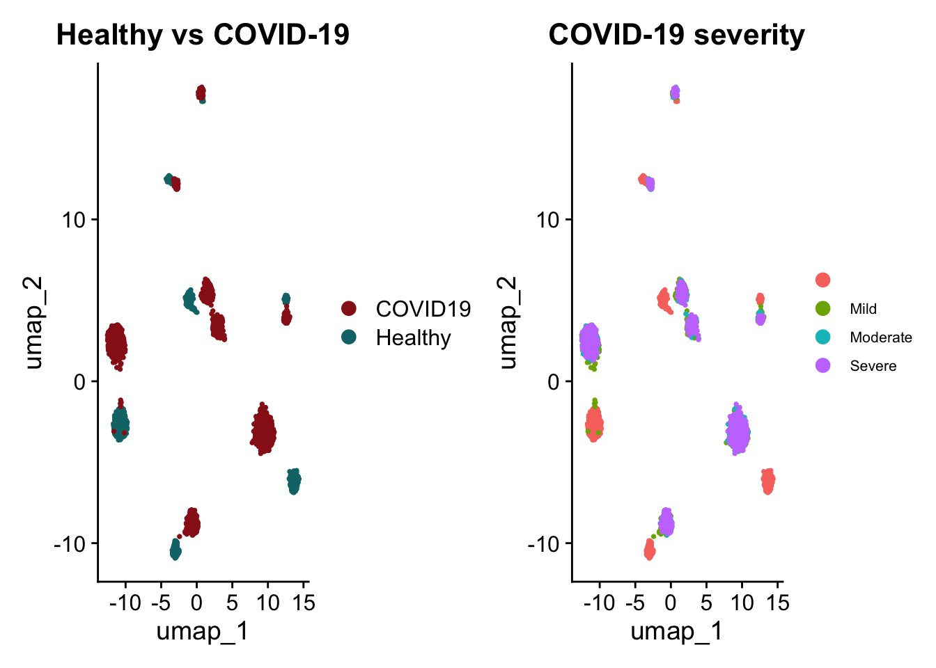
Same idea, different variable: severity by donor. The tabulation reveals the donor-condition design (which donors are Healthy vs which severity level each COVID-19 donor was assigned).

cat("\nSeverity by donor:\n")

Severity by donor:

print(table(sobj$severity, sobj$donor_id, useNA = "ifany"))

          
           Donor01 Donor02 Donor03 Donor04 Donor05 Donor06 Donor07
               350     300     350       0       0       0       0
  Mild           0       0       0     450       0       0       0
  Moderate       0       0       0       0     450       0       0
  Severe         0       0       0       0       0     550     550

4.4.8 Step 1.7 - ADT feature naming

• ADT feature names often differ from RNA gene names.
• CD3 protein != CD3E gene. CD8a protein != CD8A gene.
• This mismatch is a frequent source of confusion.

cat("ADT protein names:\n")

ADT protein names:

print(rownames(sobj[["ADT"]]))

 [1] "CD3"    "CD4"    "CD8a"   "CD14"   "CD16"   "CD19"   "CD20"   "CD25"  
 [9] "CD27"   "CD38"   "CD45RA" "CD45RO" "CD56"   "CD57"   "CD62L"  "CD69"  
[17] "CD86"   "CD127"  "CD197"  "PD1"    "TIGIT"  "LAG3"   "IgD"    "HLADR" 

cat("\nRNA marker names for comparison:\n")

RNA marker names for comparison:

rna_markers <- c("CD3E", "CD4", "CD8A", "CD14", "CD19", "NCAM1")
cat(rna_markers, "\n")

CD3E CD4 CD8A CD14 CD19 NCAM1 

cat("\nImportant: 'CD8a' in ADT vs 'CD8A' in RNA.\n")

Important: 'CD8a' in ADT vs 'CD8A' in RNA.

cat("FetchData() handles this transparently, but FeaturePlot()\n")

FetchData() handles this transparently, but FeaturePlot()

cat("requires you to be on the correct DefaultAssay first.\n")

requires you to be on the correct DefaultAssay first.

Demonstrate: what happens when you try to access an ADT feature using the RNA gene name:

cat("\nDoes 'CD8A' exist in ADT?\n")

Does 'CD8A' exist in ADT?

cat("'CD8A' in ADT rownames:", "CD8A" %in% rownames(sobj[["ADT"]]), "\n")

'CD8A' in ADT rownames: FALSE 

cat("'CD8a' in ADT rownames:", "CD8a" %in% rownames(sobj[["ADT"]]), "\n")

'CD8a' in ADT rownames: TRUE 

4.4.9 Step 1.8 - Marker stored under an alias

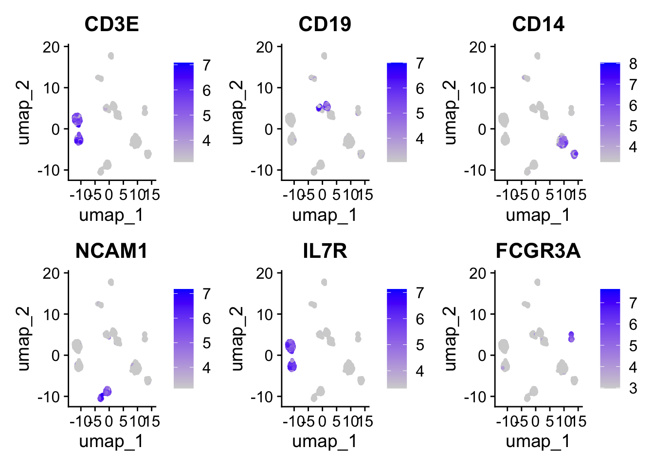
Gene symbols have synonyms: NCAM1 = CD56, FCGR3A = CD16, MS4A1 = CD20. If an object stores a gene under its alias, FeaturePlot("FCGR3A") returns “feature not found” and the marker reads as absent when the data are intact.

Confirm canonical markers exist under their expected symbol before plotting or annotating.

canonical <- c("CD3E", "CD4", "CD8A", "CD14", "CD19", "MS4A1", "NCAM1", "FCGR3A")
present   <- canonical %in% rownames(sobj[["RNA"]])

cat("Canonical RNA markers present under expected symbol:\n")

Canonical RNA markers present under expected symbol:

for (i in seq_along(canonical))
  cat(sprintf("  %-8s %s\n", canonical[i], ifelse(present[i], "OK", "MISSING")))

  CD3E     OK
  CD4      OK
  CD8A     OK
  CD14     OK
  CD19     OK
  MS4A1    OK
  NCAM1    OK
  FCGR3A   OK

If something is MISSING, search for known aliases in the rownames

aliases <- list(FCGR3A = "CD16", NCAM1 = "CD56", MS4A1 = "CD20")
missing <- canonical[!present]
if (length(missing) > 0) {
  cat("\nMISSING markers detected. Searching for aliases:\n")
  rna_counts <- LayerData(sobj, assay = "RNA", layer = "counts")
  rn <- rownames(rna_counts)
  changed <- FALSE
  for (m in missing) {
    al <- aliases[[m]]
    if (!is.null(al) && al %in% rn) {
      cat(sprintf("  %s is stored as alias '%s'. Renaming back.\n", m, al))
      rn[rn == al] <- m
      changed <- TRUE
    }
  }
  if (changed) {
    # v5-safe rename: rebuild the RNA assay from counts with corrected names.
    # Run before normalization (Block 4), so only the counts layer exists,
    # matching the structure of the assay it replaces. suppressWarnings()
    # wraps the assignment itself, since any "different features" notice
    # would come from the [[<- replacement method, not from
    # CreateAssay5Object().
    rownames(rna_counts) <- rn
    new_rna_assay <- CreateAssay5Object(counts = rna_counts)
    suppressWarnings(sobj[["RNA"]] <- new_rna_assay)
    DefaultAssay(sobj) <- "RNA"
  }
  cat("\nAfter fix, all canonical markers present:",
      all(canonical %in% rownames(sobj[["RNA"]])), "\n")
}

TipQUESTION 1.8

What other RNA aliases would you check for routinely in a PBMC dataset?

TipANSWER

Common alias pairs: MS4A1/CD20 (B cells), NCAM1/CD56 (NK), FCGR3A/CD16 (NK and ncMonocyte), ITGAX/CD11c (DC, mono), ITGAM/CD11b (myeloid), PTPRC/CD45 (pan-immune), IL3RA/CD123 (pDC, basophil), CD3E/CD3, CD8A/CD8a (case matters: RNA upper, ADT lower), FOXP3 (Treg), FCER1A (DC). Defensive habit: keep a list of canonical PBMC markers and run %in% rownames(sobj[['RNA']]) at the start of every annotation step.

LIVE DEMO:

canonical <- c("CD3E","CD3D","CD8A","CD4","MS4A1","CD79A","NCAM1",
               "FCGR3A","CD14","LYZ","FOXP3","FCER1A","KLRD1")
data.frame(marker = canonical,
           present = canonical %in% rownames(sobj[["RNA"]]))

   marker present
1    CD3E    TRUE
2    CD3D    TRUE
3    CD8A    TRUE
4     CD4    TRUE
5   MS4A1    TRUE
6   CD79A    TRUE
7   NCAM1    TRUE
8  FCGR3A    TRUE
9    CD14    TRUE
10    LYZ    TRUE
11  FOXP3    TRUE
12 FCER1A    TRUE
13  KLRD1    TRUE

# Check aliases for missing ones:
aliases <- c(MS4A1="CD20", NCAM1="CD56", FCGR3A="CD16")

4.5 Block 2 - Quality control metrics (RNA)

Goal: Compute QC metrics, look at their distributions across donors, and filter cells using thresholds chosen from the data, not from a tutorial.

4.5.1 Step 2.1 - Compute QC metrics

• Mitochondrial fraction (percent.mt) is a death/stress indicator.
• Ribosomal fraction (percent.ribo) flags cells dominated by housekeeping transcripts.

sobj[["percent.mt"]]   <- PercentageFeatureSet(sobj, pattern = "^MT-")
sobj[["percent.ribo"]] <- PercentageFeatureSet(sobj, pattern = "^RP[SL]")

summary(sobj@meta.data[, c("nFeature_RNA", "nCount_RNA", "percent.mt")])

  nFeature_RNA     nCount_RNA      percent.mt    
 Min.   :27.00   Min.   :172.0   Min.   : 0.000  
 1st Qu.:43.00   1st Qu.:381.0   1st Qu.: 2.788  
 Median :47.00   Median :451.0   Median : 5.290  
 Mean   :47.46   Mean   :451.8   Mean   : 6.463  
 3rd Qu.:52.00   3rd Qu.:517.0   3rd Qu.: 8.853  
 Max.   :69.00   Max.   :844.0   Max.   :28.605  

head(sobj@meta.data, 10)

           orig.ident nCount_RNA nFeature_RNA percent.mt donor_id condition
CELL000001    Donor01        336           36  18.154762  Donor01   Healthy
CELL000011    Donor01        344           40  15.116279  Donor01   Healthy
CELL000021    Donor01        426           39   0.000000  Donor01   Healthy
CELL000031    Donor01        330           35   3.333333  Donor01   Healthy
CELL000041    Donor01        473           51   5.073996  Donor01   Healthy
CELL000051    Donor01        488           47   9.631148  Donor01   Healthy
CELL000061    Donor01        413           55  12.106538  Donor01   Healthy
CELL000071    Donor01        294           42  15.986395  Donor01   Healthy
CELL000081    Donor01        455           36   3.956044  Donor01   Healthy
CELL000091    Donor01        336           47   5.357143  Donor01   Healthy
           severity age  cell_type nCount_ADT nFeature_ADT percent.ribo
CELL000001           35     NKcell        182           16     46.13095
CELL000011           35         DC        202           18     64.53488
CELL000021           35      Bcell        265           14     66.66667
CELL000031           35   Monocyte        135           10     60.90909
CELL000041           35   CD4Tcell        199           16     39.74630
CELL000051           35   CD4Tcell        133           16     48.36066
CELL000061           35   CD4Tcell        209           15     39.46731
CELL000071           35 ncMonocyte        141           18     59.86395
CELL000081           35   Monocyte        150           16     58.24176
CELL000091           35      Bcell        280            9     52.08333
           RNA_snn_res.0.5 seurat_clusters
CELL000001               8               8
CELL000011               9               9
CELL000021              10              10
CELL000031               5               5
CELL000041               2               2
CELL000051               2               2
CELL000061               2               2
CELL000071               7               7
CELL000081               5               5
CELL000091              10              10

4.5.2 Step 2.2 | Sanity check: did percent.mt actually compute?

• percent.mt depends entirely on the ‘^MT-’ pattern matching real gene names.

This is worth confirming explicitly rather than assuming it worked: a renamed or missing MT- prefix (which is exactly what the injected object simulates) returns percent.mt = 0 for every cell, and any filter based on it then either does nothing or rejects every cell.

mt_genes <- grep("^MT-", rownames(sobj), value = TRUE)
cat("Genes matching '^MT-':", length(mt_genes), "\n")

Genes matching '^MT-': 9 

if (length(mt_genes) > 0) print(mt_genes)

[1] "MT-CO1"  "MT-CO2"  "MT-CO3"  "MT-ND1"  "MT-ND2"  "MT-ATP6" "MT-CYB" 
[8] "MT-RNR1" "MT-RNR2"

cat("\nAre rownames symbols or Ensembl IDs? First 5 rownames:\n")

Are rownames symbols or Ensembl IDs? First 5 rownames:

print(head(rownames(sobj), 5))

[1] "CD3E" "CD3D" "CD3G" "CD4"  "CD8A"

cat("\nmax(percent.mt):", round(max(sobj$percent.mt), 4), "\n")

max(percent.mt): 28.6052 

if (max(sobj$percent.mt) == 0) {
  cat("\nWARNING: percent.mt is 0 for all cells. The '^MT-' pattern matched\n")
  cat("no genes. Do NOT filter on percent.mt here: it is uninformative in\n")
  cat("this panel. Report this limitation; do not claim an mt-based QC.\n")
} else {
  cat("MT- pattern matched", length(mt_genes), "genes. percent.mt is usable.\n")
}

MT- pattern matched 9 genes. percent.mt is usable.

TipQUESTION 2.2

If max(percent.mt) is 0 across every cell, what are the two possible explanations, and how do you tell them apart?

TipANSWER

Explanation 1 (almost always): the MT- pattern matched no genes because mitochondrial symbols use a different prefix (mt-, Mt-, MTX, or a non-human reference). Diagnostic: grep('^MT-', rownames(sobj)) returns character(0). Inspect head(rownames(sobj)) and look for the actual prefix. Explanation 2 (implausible): cells filtered upstream so aggressively that no MT transcripts remain. The pattern mismatch is the realistic case. The injected dataset renames MT- genes to MTX- to trip this exact failure.

LIVE DEMO:

grep("^MT-", rownames(sobj), value = TRUE)

[1] "MT-CO1"  "MT-CO2"  "MT-CO3"  "MT-ND1"  "MT-ND2"  "MT-ATP6" "MT-CYB" 
[8] "MT-RNR1" "MT-RNR2"

grep("^mt-", rownames(sobj), value = TRUE)

character(0)

grep("^MTX", rownames(sobj), value = TRUE)

character(0)

head(rownames(sobj), 20)

 [1] "CD3E"   "CD3D"   "CD3G"   "CD4"    "CD8A"   "CD8B"   "IL7R"   "CCR7"  
 [9] "TCF7"   "SELL"   "FOXP3"  "IL2RA"  "PDCD1"  "LAG3"   "HAVCR2" "CD19"  
[17] "MS4A1"  "CD79A"  "CD79B"  "IGHM"  

summary(sobj$percent.mt)

   Min. 1st Qu.  Median    Mean 3rd Qu.    Max. 
  0.000   2.788   5.290   6.463   8.853  28.605 

4.5.3 Step 2.3 - Visualize QC distributions

VlnPlot(sobj,
        features = c("nFeature_RNA", "nCount_RNA", "percent.mt"),
        ncol = 3, pt.size = 0.05, alpha = 0.3)

p1 <- FeatureScatter(sobj, "nCount_RNA", "nFeature_RNA") +
  ggtitle("Counts vs genes detected") +
  theme(plot.title = element_text(size = 10))
p2 <- FeatureScatter(sobj, "nCount_RNA", "percent.mt") +
  ggtitle("Counts vs mitochondrial %") +
  theme(plot.title = element_text(size = 10))
p1 | p2

4.5.4 Step 2.4 - Outlier detection

Cells that are high in nFeature relative to nCount might be doublets.

• Low nCount with low nFeature = empty droplet.
• High percent.mt alone = stressed/dying cell.

Cells that are potential outliers: nFeature > 2 SD above mean

mean_feat <- mean(sobj$nFeature_RNA)
sd_feat   <- sd(sobj$nFeature_RNA)
high_feat <- sum(sobj$nFeature_RNA > mean_feat + 2 * sd_feat)
cat("Cells with nFeature > mean + 2 SD (potential doublets):",
    high_feat, "\n")

Cells with nFeature > mean + 2 SD (potential doublets): 58 

Cells with high mt: > 95th percentile

mt_95 <- quantile(sobj$percent.mt, 0.95)
high_mt <- sum(sobj$percent.mt > mt_95)
cat("Cells with percent.mt > 95th percentile:", high_mt, "\n")

Cells with percent.mt > 95th percentile: 150 

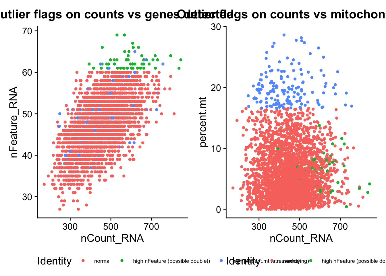
The two counts above are easy to compute and easy to misread: a count by itself does not show whether the flagged cells form a clear, separable group, or whether the threshold cut through the middle of a continuous distribution. Flag both categories on the metadata and plot them directly against the same axes used in Step 2.3 (Section 4.5.3), so the outliers are visible as points, not just as a number.

sobj$outlier_flag <- "normal"
sobj$outlier_flag[sobj$nFeature_RNA > mean_feat + 2 * sd_feat] <- "high nFeature (possible doublet)"
sobj$outlier_flag[sobj$percent.mt > mt_95]                     <- "high percent.mt (stressed/dying)"
sobj$outlier_flag <- factor(sobj$outlier_flag,
                            levels = c("normal", "high nFeature (possible doublet)",
                                       "high percent.mt (stressed/dying)"))

p_out1 <- FeatureScatter(sobj, "nCount_RNA", "nFeature_RNA", group.by = "outlier_flag") +
  ggtitle("Outlier flags on counts vs genes detected") +
  theme(legend.position = "bottom", legend.text = element_text(size = 7))

p_out2 <- FeatureScatter(sobj, "nCount_RNA", "percent.mt", group.by = "outlier_flag") +
  ggtitle("Outlier flags on counts vs mitochondrial %") +
  theme(legend.position = "bottom", legend.text = element_text(size = 7))

p_out1 | p_out2

TipQUESTION 2.4

Looking at the two plots, do the high-nFeature cells and the high-percent.mt cells occupy distinct regions, or do some cells qualify as both? What would a cell flagged on both axes most likely be?

TipANSWER

In most runs the two flagged groups are largely distinct: high-nFeature outliers cluster toward the right side of the nCount-vs-nFeature plot (more genes detected than the bulk of cells at a similar UMI count), while high-percent.mt outliers cluster in the upper region of the nCount-vs-percent.mt plot regardless of nFeature. Some overlap is expected and is the informative case: a cell flagged on both axes (high nFeature AND high percent.mt) is the hardest to call from a single metric. It could be a doublet that happens to also be stressed, or it could be two unrelated technical issues compounding in the same cell. The practical move is not to try to assign a single cause; flag the cell as low-confidence and let downstream steps (doublet scoring in Block 3, annotation confidence in Block 5, Section 4.8) make the final call with more evidence.

LIVE DEMO:

table(sobj$outlier_flag)

                          normal high nFeature (possible doublet) 
                            2797                               53 
high percent.mt (stressed/dying) 
                             150 

# Cells flagged on both definitions (recompute the masks to check overlap):
both <- (sobj$nFeature_RNA > mean_feat + 2*sd_feat) & (sobj$percent.mt > mt_95)
sum(both)

[1] 5

Distribution per condition: is mt% elevated in COVID-19?

cat("\nMedian percent.mt by condition:\n")

Median percent.mt by condition:

sobj@meta.data %>%
  group_by(condition) %>%
  summarise(median_mt = round(median(percent.mt), 2),
            mean_mt   = round(mean(percent.mt),   2),
            .groups   = "drop") %>%
  print()

# A tibble: 2 × 3
  condition median_mt mean_mt
  <chr>         <dbl>   <dbl>
1 COVID19        5.05    6.08
2 Healthy        5.74    7.23

4.5.5 Step 2.5 - Wrong filter: tutorial thresholds applied blindly

Standard tutorial thresholds (nFeature > 200 & < 6000, percent.mt < 5%) are inherited from full 10x experiments with ~33,000 genes. This dataset is a 500-gene subset for teaching purposes. Applying the tutorial cutoffs deletes every cell.

# >>> DELIBERATE ERROR - read the message, then continue. <<<
try({
  sobj_filt <- subset(
    sobj,
    subset = nFeature_RNA > 200 &
             nFeature_RNA < 5000 &
             percent.mt   < 20
  )
})

Error in subset(sobj, subset = nFeature_RNA > 200 & nFeature_RNA < 5000 &  : 
  No cells found

Important

“No cells found” is the canonical result of copying thresholds from a tutorial without checking your own data distribution. The threshold nFeature_RNA > 200 was calibrated for a transcriptome of ~33,000 genes where cells typically detect 2,000-3,000 genes. In a 500-gene panel, most cells detect 50-150 genes. The filter removes every single cell.

TipQUESTION 2.5

Which of the three filter parameters above is the most wrong for this 500-gene dataset, and what value would you try first? Run quantile(sobj$nFeature_RNA, c(0.05, 0.95)) to see the actual range before proposing a number.

TipANSWER

nFeature_RNA > 200 is the most wrong. The tutorial value 200 was calibrated for ~33,000 features where cells detect 2,000-3,000 genes; here the 500-gene panel produces 50-150 detected per cell, so a 200 floor removes essentially all cells. Reasonable starting threshold here is the 5th percentile of nFeature_RNA, typically near 30-50. nFeature_RNA < 6000 is technically fine because no cell has near 6000 features in a 500-gene panel; it just does nothing. percent.mt < 5 is borderline; effect depends on whether the MT pattern matched.

LIVE DEMO:

quantile(sobj$nFeature_RNA, c(0.05, 0.50, 0.95))

 5% 50% 95% 
 37  47  58 

summary(sobj$nFeature_RNA)

   Min. 1st Qu.  Median    Mean 3rd Qu.    Max. 
  27.00   43.00   47.00   47.46   52.00   69.00 

lo <- quantile(sobj$nFeature_RNA, 0.05)
hi <- quantile(sobj$nFeature_RNA, 0.95)
subset(sobj, subset = nFeature_RNA >= lo & nFeature_RNA <= hi)

An object of class Seurat 
524 features across 2712 samples within 2 assays 
Active assay: RNA (500 features, 500 variable features)
 3 layers present: counts, data, scale.data
 1 other assay present: ADT
 2 dimensional reductions calculated: pca, umap

A reasonable first guess for this panel: nFeature_RNA > 50. Try it and see how many cells survive, before moving to the fully data-driven thresholds in Step 2.6 and 2.7 (Section 4.5.6, Section 4.5.7).

n_above_50 <- sum(sobj$nFeature_RNA > 50)
cat("Cells with nFeature_RNA > 50:", n_above_50,
    sprintf("(%.1f%% of total)\n", 100 * n_above_50 / ncol(sobj)))

Cells with nFeature_RNA > 50: 982 (32.7% of total)

4.5.6 Step 2.6 - Compare tutorial vs data-driven thresholds

cat("--- Published thresholds (full 10x, 33k genes) ---\n")

--- Published thresholds (full 10x, 33k genes) ---

cat("  nFeature_RNA > 200   removes empty droplets\n")

  nFeature_RNA > 200   removes empty droplets

cat("  nFeature_RNA < 5000  removes likely doublets\n")

  nFeature_RNA < 5000  removes likely doublets

cat("  percent.mt   < 20%   removes dead/stressed cells\n\n")

  percent.mt   < 20%   removes dead/stressed cells

cat("--- This dataset (500 genes) ---\n")

--- This dataset (500 genes) ---

print(round(quantile(sobj$nFeature_RNA,
      probs = c(0.01, 0.05, 0.25, 0.5, 0.75, 0.95, 0.99))))

 1%  5% 25% 50% 75% 95% 99% 
 33  37  43  47  52  58  62 

cat("\n--- Data-driven thresholds ---\n")

--- Data-driven thresholds ---

min_features <- max(10, round(quantile(sobj$nFeature_RNA, 0.02)))
max_features <- round(quantile(sobj$nFeature_RNA, 0.98))
max_mt       <- round(quantile(sobj$percent.mt,   0.95), 1)

cat("  nFeature_RNA > ", min_features, "  (same intent: empty droplets)\n")

  nFeature_RNA >  34   (same intent: empty droplets)

cat("  nFeature_RNA < ", max_features, " (same intent: doublets)\n")

  nFeature_RNA <  60  (same intent: doublets)

cat("  percent.mt   < ", max_mt, "%  (same intent: dead cells)\n")

  percent.mt   <  16.5 %  (same intent: dead cells)

4.5.7 Step 2.7 - Apply data-driven thresholds

cat("Cells before filtering:", ncol(sobj), "\n")

Cells before filtering: 3000 

sobj_filt <- tryCatch(
  subset(
    sobj,
    subset = nFeature_RNA > min_features &
             nFeature_RNA < max_features &
             percent.mt   < max_mt
  ),
  error = function(e) {
    cat("\nsubset() failed:", conditionMessage(e), "\n")
    cat("This means the three thresholds together match zero cells.\n")
    cat("Check each threshold individually before combining them:\n")
    cat("  > min_features:", sum(sobj$nFeature_RNA > min_features), "cells\n")
    cat("  < max_features:", sum(sobj$nFeature_RNA < max_features), "cells\n")
    cat("  < max_mt      :", sum(sobj$percent.mt   < max_mt),       "cells\n")
    stop(e)
  }
)

cat("Cells after filtering :", ncol(sobj_filt), "\n")

Cells after filtering : 2683 

cat("Cells removed         :", ncol(sobj) - ncol(sobj_filt), "\n")

Cells removed         : 317 

cat("Retention rate        :",
    round(ncol(sobj_filt) / ncol(sobj) * 100, 1), "%\n")

Retention rate        : 89.4 %

if (ncol(sobj_filt) < 500) {
  cat("\nWARNING: fewer than 500 cells remaining.\n")
  cat("Options: relax max_mt or lower min_features,\n")
  cat("or request pre-filtered matrices from GEO.\n")
} else {
  cat("\nCell count adequate for downstream analysis.\n")
}

Cell count adequate for downstream analysis.

TipQUESTION 2.7

How would your thresholds change if the dataset had ~33,000 genes instead of 500?

TipANSWER

Thresholds on detected-feature counts scale roughly linearly with feature space, but thresholds on quality metrics (percent.mt, percent.ribo) do not. For 33,000 genes: nFeature_RNA lower 200-500, upper 5,000-8,000; nCount_RNA upper into tens of thousands. percent.mt is independent of feature count (a fraction of UMIs), so 10-20% upper bound is tissue-driven, not size-driven. Always inspect the distribution before fixing any number.

LIVE DEMO:

p1 <- VlnPlot(sobj, "nFeature_RNA", group.by="donor_id") + ggtitle("500-gene panel")
print(p1)

4.5.8 Step 2.8 - Silent failure: percent.mt as fraction vs as percentage

A common silent failure: someone copied a threshold from a tutorial that used percent.mt expressed as a FRACTION (0 to 1), but Seurat returns percent.mt as a PERCENTAGE (0 to 100). The filter looks right and runs without error, but removes nearly every cell.

# >>> DELIBERATE ERROR - read the message, then continue. <<<
try({
  # This filter expects 5 percent (i.e. percent.mt < 5). Written as 0.05 it
  # means "less than 0.05 percent", which removes almost everything.
  sobj_fraction <- subset(sobj, subset = percent.mt < 0.05)
  cat("Cells passing 'percent.mt < 0.05' filter :", ncol(sobj_fraction), "\n")
})

Cells passing 'percent.mt < 0.05' filter : 22 

cat("Compare to the correct threshold (percent.mt < 5):\n")

Compare to the correct threshold (percent.mt < 5):

sobj_pct <- subset(sobj, subset = percent.mt < 5)
cat("Cells passing 'percent.mt < 5' filter    :", ncol(sobj_pct), "\n")

Cells passing 'percent.mt < 5' filter    : 1423 

TipQUESTION 2.8

Is your dataset’s percent.mt distribution closer to a fraction or a percentage? Run summary(sobj$percent.mt) to confirm and remember this trap when reading code from other groups.

TipANSWER

It is a percentage. PercentageFeatureSet returns values on a 0-100 scale. A real PBMC dataset typically sits between 0 and 15 percent mitochondrial. If you see values between 0 and 1, you are looking at a fraction encoding (someone divided by 100), and any threshold expressed as a percentage will be wrong. Diagnostic: summary(sobj$percent.mt) - if max is under 1, it is a fraction; otherwise it is a percentage.

LIVE DEMO:

summary(sobj$percent.mt)

   Min. 1st Qu.  Median    Mean 3rd Qu.    Max. 
  0.000   2.788   5.290   6.463   8.853  28.605 

4.5.9 Step 2.9 - Spot the bug

Read the code below CAREFULLY before running it. What is wrong with it?

Write your answer as a comment on the next line.

covid_cells <- subset(sobj_filt, subset = condition == "COVID")

Error in `subset()`:
! No cells found

Your answer:

REVEAL: the condition value in this dataset is “COVID19”, not “COVID”. - subset() returns zero cells without any error. Always inspect the unique values of a categorical column before subsetting on it.

cat("Unique values of condition in this dataset:\n")

Unique values of condition in this dataset:

print(unique(sobj_filt$condition))

[1] "Healthy" "COVID19"

TipTip

Habit: print unique() of a factor or character column before referencing any specific value in subset() or filter().

4.6 Block 3 - Doublet detection

Goal: Identify and remove technical doublets that survive QC thresholds. + scDblFinder simulates artificial doublets and scores each real cell against them. The result is a doublet class label and a numeric score per cell.

4.6.1 Step 3.1 - Run scDblFinder

library(scDblFinder)

Both packages are already loaded from Block 0; no need to library() again.

• scDblFinder calls xgboost internally; recent xgboost versions emit deprecation warnings unrelated to our analysis. Wrap the call to keep the console focused on the actual result.

set.seed(42)
sce <- SingleCellExperiment(
  assays = list(counts = LayerData(sobj_filt, assay = "RNA", layer = "counts"))
)
sce <- suppressWarnings(scDblFinder(sce))

Creating ~2147 artificial doublets...

Dimensional reduction

Evaluating kNN...

Training model...

iter=0, 78 cells excluded from training.

iter=1, 83 cells excluded from training.

iter=2, 92 cells excluded from training.

Threshold found:0.377

10 (0.4%) doublets called

sobj_filt$scDblFinder.class <- sce$scDblFinder.class
sobj_filt$scDblFinder.score <- sce$scDblFinder.score

cat("Doublet classification:\n")

Doublet classification:

print(table(sobj_filt$scDblFinder.class))

singlet doublet 
   2673      10 

cat("\nDoublet rate:",
    round(mean(sobj_filt$scDblFinder.class == "doublet") * 100, 1), "%\n")

Doublet rate: 0.4 %

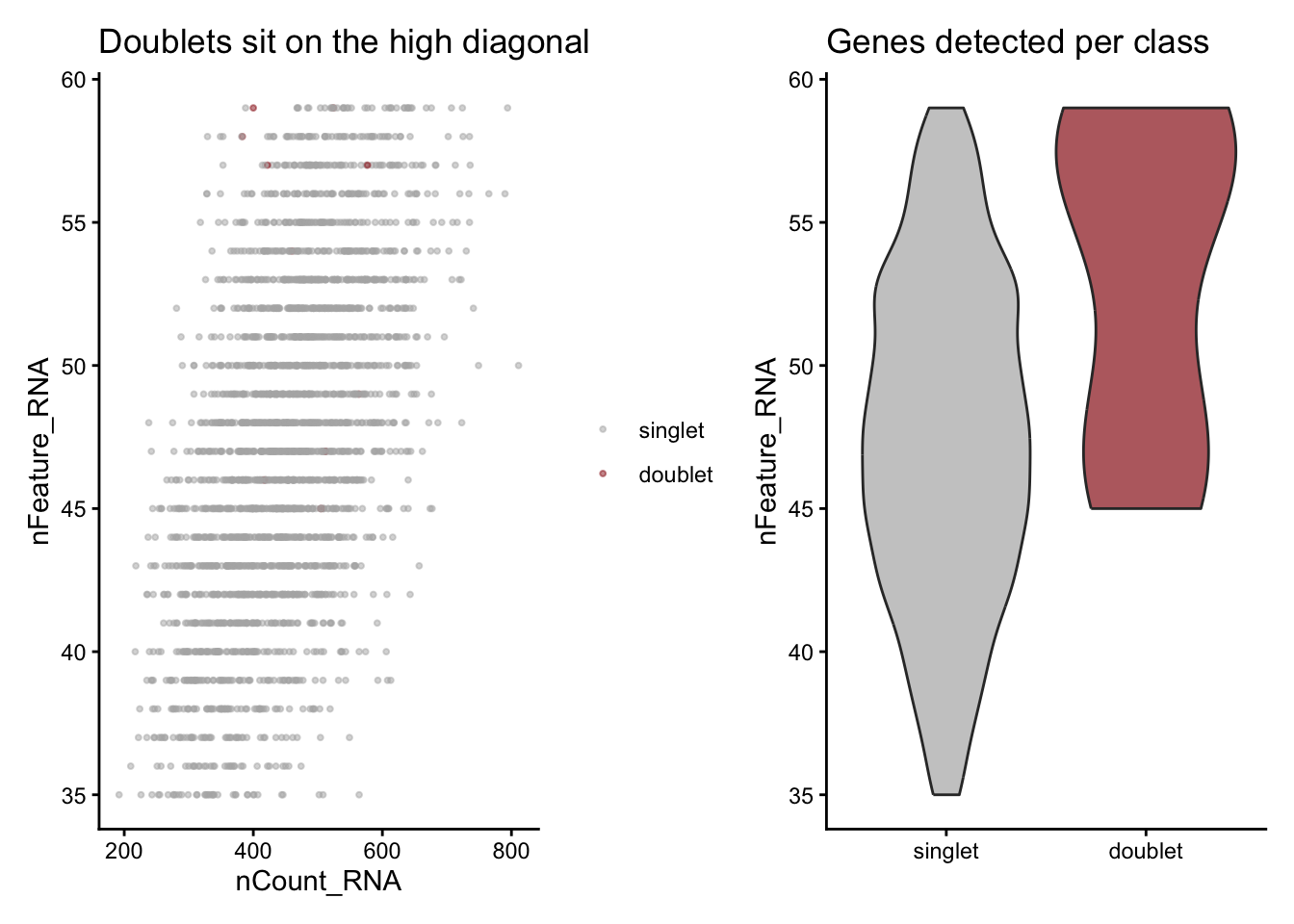
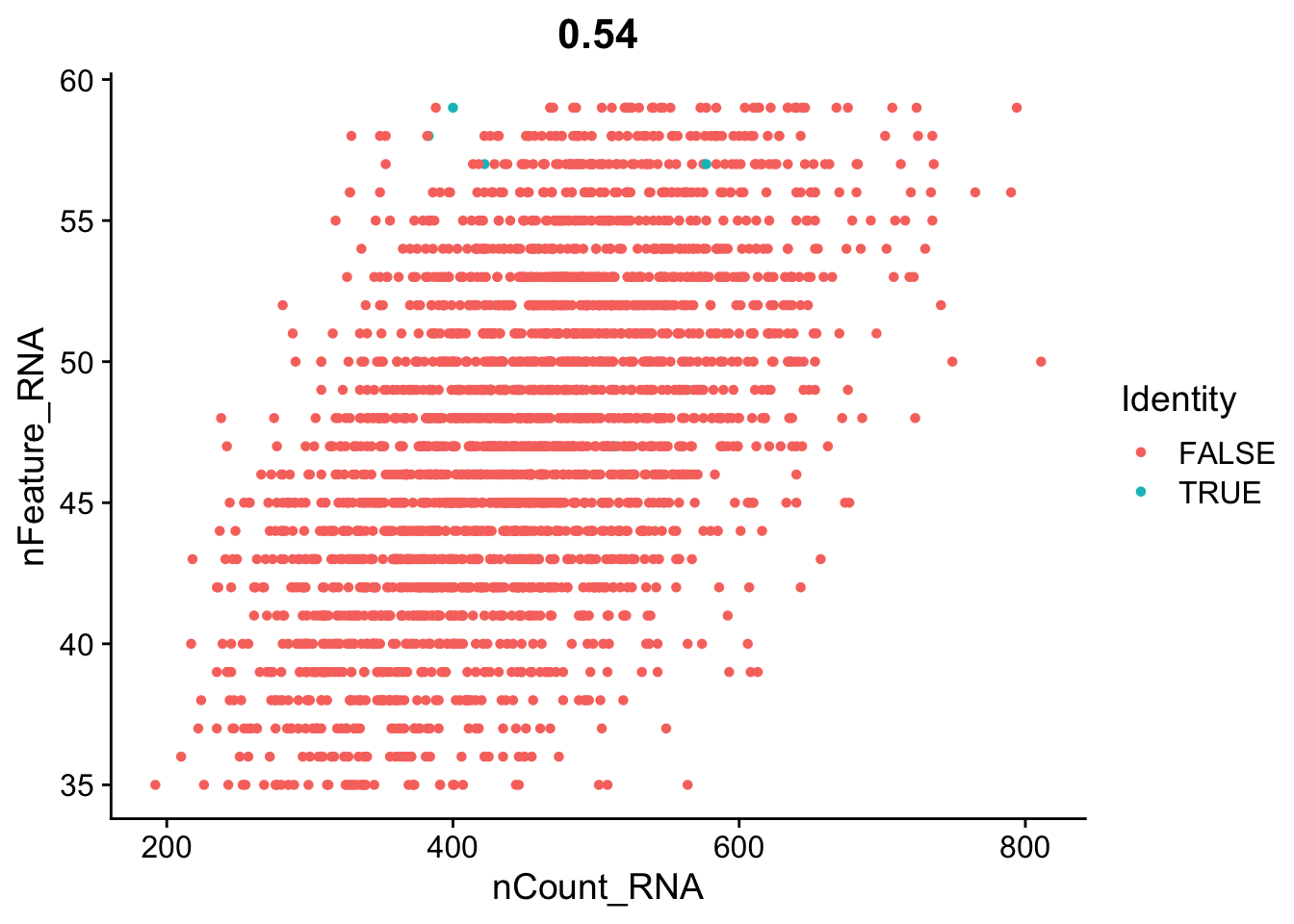
4.6.2 Step 3.2 - Where do flagged doublets sit on the QC scatter?

df <- sobj_filt@meta.data
p1 <- ggplot(df, aes(nCount_RNA, nFeature_RNA, color = scDblFinder.class)) +
  geom_point(alpha = 0.5, size = 0.7) +
  scale_color_manual(values = c("singlet" = "grey70", "doublet" = "#991b1b")) +
  labs(title = "Doublets sit on the high diagonal", color = NULL) +
  theme_classic(base_size = 11)

p2 <- ggplot(df, aes(scDblFinder.class, nFeature_RNA, fill = scDblFinder.class)) +
  geom_violin(alpha = 0.7) +
  scale_fill_manual(values = c("singlet" = "grey70", "doublet" = "#991b1b")) +
  labs(title = "Genes detected per class", x = NULL) +
  theme_classic(base_size = 11) + theme(legend.position = "none")

p1 | p2

TipQUESTION 3.2

Why is it expected that doublets do NOT all sit at the very top of nCount_RNA? What does that imply about using nCount thresholds alone to remove doublets?

TipANSWER

A doublet of two similar cells (two CD4 T cells, two monocytes) has roughly the same transcriptional content as one cell, just at higher capture; depending on capture efficiency and library prep, its nCount may sit anywhere inside the singlet distribution. Easy-to-detect doublets are heterotypic (T + monocyte, B + DC) because they have hybrid transcriptomes. Hard-to-detect doublets are homotypic. nCount thresholds catch only the very high tail. scDblFinder catches the transcriptional hybrids that thresholds miss. Implication: nCount filtering is necessary but not sufficient.

LIVE DEMO:

sobj_filt$is_dbl <- sce$scDblFinder.class == "doublet"
FeatureScatter(sobj_filt, "nCount_RNA", "nFeature_RNA", group.by = "is_dbl")

PLOT / OUTPUT: FeatureScatter() colored by doublet class; doublets distributed across the cloud, not just the top

4.6.3 Step 3.3 - Remove doublets

cat("Cells before doublet removal:", ncol(sobj_filt), "\n")

Cells before doublet removal: 2683 

sobj_filt <- subset(sobj_filt, subset = scDblFinder.class == "singlet")
cat("Cells after doublet removal :", ncol(sobj_filt), "\n")

Cells after doublet removal : 2673 

4.6.4 Step 3.4 - Re-inspect the object after QC and doublet removal

After every step that mutates the object, confirm what you now have. Silent bugs surface only when the object is re-inspected, not when it is re-used.

cat("Object after QC + doublet removal:\n")

Object after QC + doublet removal:

print(sobj_filt)

An object of class Seurat 
524 features across 2673 samples within 2 assays 
Active assay: RNA (500 features, 500 variable features)
 3 layers present: counts, data, scale.data
 1 other assay present: ADT
 2 dimensional reductions calculated: pca, umap

cat("\nCells lost   :", ncol(sobj) - ncol(sobj_filt), "\n")

Cells lost   : 327 

cat("Cells kept   :", ncol(sobj_filt), "\n")

Cells kept   : 2673 

cat("Median genes :", median(sobj_filt$nFeature_RNA), "\n")

Median genes : 47 

cat("Median UMIs  :", median(sobj_filt$nCount_RNA), "\n")

Median UMIs  : 452 

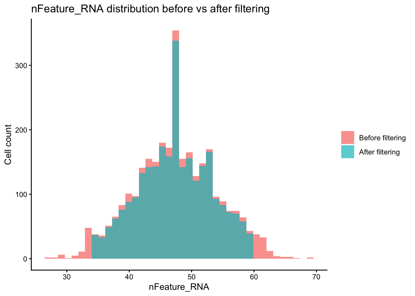
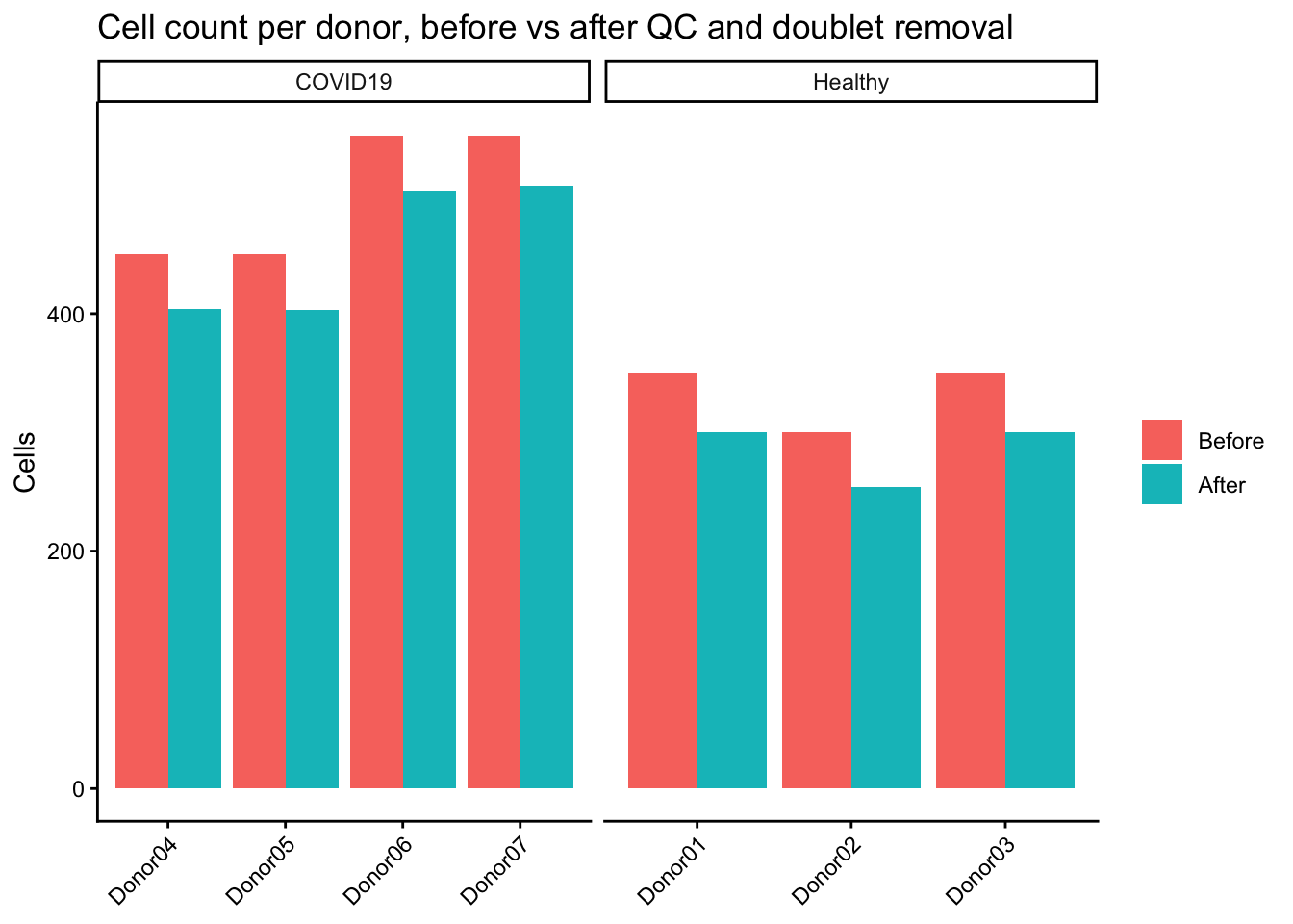
Two views of the same removal: the overall distribution shift, and the per-donor breakdown. A filter that looks reasonable in aggregate can still remove one donor almost entirely; the per-donor bar chart is what catches that before it becomes a downstream surprise.

before_after <- bind_rows(
  data.frame(nFeature_RNA = sobj$nFeature_RNA, stage = "Before filtering"),
  data.frame(nFeature_RNA = sobj_filt$nFeature_RNA, stage = "After filtering")
)
before_after$stage <- factor(before_after$stage,
                             levels = c("Before filtering", "After filtering"))

p_before_after <- ggplot(before_after, aes(x = nFeature_RNA, fill = stage)) +
  geom_histogram(bins = 40, alpha = 0.7, position = "identity") +
  labs(title = "nFeature_RNA distribution before vs after filtering",
       x = "nFeature_RNA", y = "Cell count", fill = NULL) +
  theme_classic(base_size = 11)

cell_counts <- data.frame(
  donor_id  = c(sobj$donor_id, sobj_filt$donor_id),
  condition = c(sobj$condition, sobj_filt$condition),
  stage     = rep(c("Before", "After"), c(ncol(sobj), ncol(sobj_filt)))
) %>%
  dplyr::count(donor_id, condition, stage) %>%
  dplyr::mutate(stage = factor(stage, levels = c("Before", "After")))

p_donor_counts <- ggplot(cell_counts, aes(x = donor_id, y = n, fill = stage)) +
  geom_bar(stat = "identity", position = "dodge") +
  facet_wrap(~condition, scales = "free_x") +
  labs(title = "Cell count per donor, before vs after QC and doublet removal",
       x = NULL, y = "Cells", fill = NULL) +
  theme_classic(base_size = 11) +
  theme(axis.text.x = element_text(angle = 45, hjust = 1))

p_before_after

p_donor_counts

TipQUESTION 3.4

Look at the per-donor bar chart. Did any single donor lose a much larger fraction of cells than the others? If so, is that donor-level QC variation, or a sign the filter thresholds were tuned around the majority of donors at the expense of one outlier?

TipANSWER

Compare the before/after height for each donor rather than the overall retention rate. A donor that loses a noticeably larger fraction than the rest is worth a second look before proceeding: it could be genuine biological or technical donor-level variation (a donor with systematically lower RNA quality, more dying cells, or a different processing batch), or it could mean the data-driven thresholds in Step 2.7 (Section 4.5.7), which were computed across all donors pooled together, happen to fall in a range that disproportionately penalizes one donor’s distribution. The fix is the same either way: if one donor’s loss looks extreme, compute thresholds per donor and compare, rather than assuming a single global threshold serves every donor equally. Silently losing most of one donor’s cells changes what every downstream comparison (by condition, by severity) is actually measuring.

LIVE DEMO:

cell_counts %>% group_by(donor_id) %>%
  summarise(before = sum(n[stage=="Before"]),
            after  = sum(n[stage=="After"]),
            pct_kept = round(100*after/before, 1))

# A tibble: 7 × 4
  donor_id before after pct_kept
  <chr>     <int> <int>    <dbl>
1 Donor01     350   300     85.7
2 Donor02     300   254     84.7
3 Donor03     350   300     85.7
4 Donor04     450   404     89.8
5 Donor05     450   403     89.6
6 Donor06     550   504     91.6
7 Donor07     550   508     92.4

4.7 Block 4 - Normalization, dimensionality reduction, clustering (RNA)

Goal: Take the RNA assay from raw counts to a clustered UMAP. ADT normalization is intentionally NOT done here; it belongs to Block 6 (Section 5.1) where the CITE-seq workflow starts. Keep the modalities separate until WNN.

4.7.1 Step 4.1 - Confirm the counts layer holds raw integer counts

A common silent failure: an object arrives with the data layer copied into the counts layer (already log-normalized). NormalizeData then runs on already-normalized values. The fix has to happen here, before any normalization call.

raw <- LayerData(sobj_filt, assay = "RNA", layer = "counts")
vals <- raw@x  # non-zero values
cat("Min non-zero count :", round(min(vals), 4), "\n")

Min non-zero count : 1 

cat("Max count          :", round(max(vals), 2), "\n")

Max count          : 145 

cat("All integers?      :", all(vals == round(vals)), "\n")

All integers?      : TRUE 

if (!all(vals == round(vals))) {
  cat("\nWARNING: counts layer contains non-integer values.\n")
  cat("This is not raw counts. Do NOT run NormalizeData on it.\n")
  cat("Obtain the original count matrix before continuing.\n")
} else {
  cat("\nCounts layer looks like raw counts. Safe to normalize.\n")
}

Counts layer looks like raw counts. Safe to normalize.

# >>> DELIBERATE ERROR - read the message, then continue. <<<
# What does this check look like on a CORRUPTED counts layer?
# Simulate: a well-meaning collaborator copied the data layer back into counts
# "for consistency". Run the integrity check on that simulated layer and
# compare with the real one above.
try({
  # Build a fake assay where counts holds log-normalized values
  fake_data   <- LayerData(sobj_filt, assay = "RNA", layer = "counts")
  fake_data@x <- log1p(fake_data@x / 1e4)  # roughly what LogNormalize produces
  fake_assay  <- CreateAssay5Object(counts = fake_data)
  fake_vals   <- LayerData(fake_assay, layer = "counts")@x

  cat("\n--- Integrity check on a CORRUPTED counts layer ---\n")
  cat("Min non-zero :", round(min(fake_vals), 4), "\n")
  cat("Max          :", round(max(fake_vals), 4), "\n")
  cat("All integers?:", all(fake_vals == round(fake_vals)), "\n")
  cat("This is what a contaminated counts layer looks like.\n")
  cat("If you see this on a real object, STOP and ask for the raw matrix.\n")
})

--- Integrity check on a CORRUPTED counts layer ---
Min non-zero : 1e-04 
Max          : 0.0144 
All integers?: FALSE 
This is what a contaminated counts layer looks like.
If you see this on a real object, STOP and ask for the raw matrix.

TipQUESTION 4.1

If integrity check fails on a real inherited object, what do you ask the collaborator for? What is the absolute minimum you need to restart the analysis from a clean state?

TipANSWER

Ask for the raw CreateSeuratObject() output, OR the original 10x Genomics output (filtered_feature_bc_matrix), OR the original .rds saved before NormalizeData was first called. Minimum need: the raw counts matrix with cell and feature names matching the rest of the metadata. Anything downstream (normalized values, PCA, UMAP, clustering, annotation) can be regenerated. Without raw counts you cannot verify any quantitative claim. Make explicit: every publication-track project should preserve a checkpoint at CreateSeuratObject, before any normalization.

LIVE DEMO:

is_integer_counts <- function(layer) {
  v <- layer@x
  is.numeric(v) && all(v >= 0) && all(v == round(v))
}
is_integer_counts(LayerData(sobj_filt, assay="RNA", layer="counts"))

[1] TRUE

4.7.2 Step 4.2 - RNA normalization: LogNormalize

sobj_filt <- NormalizeData(
  sobj_filt,
  normalization.method = "LogNormalize",
  scale.factor         = 10000
)

Normalizing layer: counts

cat("RNA normalized. Layer 'data' now populated.\n")

RNA normalized. Layer 'data' now populated.

cat("Layers present:", paste(SafeLayers(sobj_filt[["RNA"]]), collapse = ", "), "\n")

Layers present: counts, data, scale.data 

Verify: log-normalized values should be non-negative

data_layer <- LayerData(sobj_filt, assay = "RNA", layer = "data")
cat("Any negative values in RNA data layer:", any(data_layer < 0), "\n")

Any negative values in RNA data layer: FALSE 

cat("Max value in RNA data layer          :",
    round(max(data_layer@x), 2), "\n")

Max value in RNA data layer          : 8.03 

TipQUESTION 4.2

Why is LogNormalize applied to RNA but CLR (margin = 2) used for ADT? What property of each modality drives the difference?

TipANSWER

RNA: variable per-cell library size (10s to 10,000s of UMIs), gene counts heavily right-skewed, very sparse. LogNormalize divides each cell’s counts by its total, multiplies by 10,000, then takes log1p. ADT: per-cell antibody load is much more uniform across cells (every cell got the same staining mix), proteins are not sparse, and the meaningful signal is relative abundance of one protein versus others within the same cell. CLR (centered log-ratio) with margin=2 treats each cell’s protein counts as a composition and normalizes within the cell, centering at zero. margin=1 would normalize across cells per protein, which removes the biological signal of which cells stain positive.

LIVE DEMO:

summary(LayerData(sobj_filt, assay="RNA", layer="counts")@x)

   Min. 1st Qu.  Median    Mean 3rd Qu.    Max. 
  1.000   1.000   4.000   9.541  14.000 145.000 

summary(LayerData(sobj_filt, assay="ADT", layer="counts")@x)

   Min. 1st Qu.  Median    Mean 3rd Qu.    Max. 
   1.00    1.00    1.00   10.54    2.00  294.00 

Note: RNA counts 0-200s typical; ADT counts 0-1000s typical.

4.7.3 Step 4.3 - Highly variable genes

sobj_filt <- FindVariableFeatures(
  sobj_filt,
  selection.method = "vst",
  nfeatures        = 2000
)

Finding variable features for layer counts

top10 <- head(VariableFeatures(sobj_filt), 10)
cat("Top 10 most variable genes:\n")

Top 10 most variable genes:

print(top10)

 [1] "ITGA2B" "PF4"    "GP1BB"  "TUBB1"  "PPBP"   "FCGR3A" "IRF8"   "MS4A7" 
 [9] "LYZ"    "CCR7"  

cat("\nTotal variable features selected:", length(VariableFeatures(sobj_filt)), "\n")

Total variable features selected: 500 

• Challenge: what fraction of all genes are selected as variable?

all_genes <- nrow(sobj_filt[["RNA"]])
n_var     <- length(VariableFeatures(sobj_filt))
cat("Variable fraction:", round(n_var / all_genes * 100, 1), "% of all genes\n")

Variable fraction: 100 % of all genes

4.7.4 Step 4.4 - Scale and run PCA

vars.to.regress removes the linear effect of percent.mt from each gene before scaling. This reduces the influence of cell stress/quality on the principal components.

sobj_filt <- ScaleData(
  sobj_filt,
  vars.to.regress = "percent.mt",
  verbose         = FALSE
)

sobj_filt <- RunPCA(sobj_filt, npcs = 30, verbose = FALSE)

Where do the PC coordinates live, now that PCA actually exists? Step 1.6 (Section 4.4.7) confirmed reductions were empty before this point; here are the three access patterns in practice.

cat("Reductions now available:", paste(SafeReductions(sobj_filt), collapse = ", "), "\n\n")

Reductions now available: pca, umap 

cat("Cell embeddings (cells x dims matrix), first 6 cells:\n")

Cell embeddings (cells x dims matrix), first 6 cells:

print(head(sobj_filt@reductions$pca@cell.embeddings))

                 PC_1       PC_2       PC_3     PC_4       PC_5         PC_6
CELL000011 -0.3873038  0.5668010 -0.8098380 5.706257 -8.1384301  3.928232203
CELL000021 -3.1533253 -7.3538408 -0.9866441 3.724133  2.2049994 -0.217801983
CELL000031 -2.5582802  2.4435804  3.4516301 5.465073  1.2167644 -0.002586255
CELL000041  6.4807853 -0.3325541 -0.3057807 1.854186  1.4233016  0.228833361
CELL000051  6.8346946 -0.3618520 -0.3202430 1.728192 -0.1796808 -2.190339236
CELL000061  7.3818265 -0.8512410  0.1201711 1.197970  0.7898951 -0.202019481
                 PC_7       PC_8       PC_9      PC_10      PC_11       PC_12
CELL000011  1.5609123 -1.8382579 -1.4743282 -0.2543423 -1.6961021  1.45573562
CELL000021  0.8133849 -1.1628040 -1.0338714 -0.7173800 -1.6887688 -0.97375034
CELL000031  0.6921562 -1.2557761  0.1039847 -0.2911183  0.2403640  2.13562491
CELL000041  0.6663791 -1.6453516  1.1500996  0.7569188  1.5069090  0.05940694
CELL000051  1.7836942  0.9288688  0.7521531  1.1371763 -0.6041043 -0.31607613
CELL000061 -0.8747301  1.8619551  0.1415833 -2.5307814 -0.3209138  2.32895553
                PC_13         PC_14      PC_15      PC_16      PC_17
CELL000011 -1.1607951 -2.1497776263 -1.6291037  0.2034311  0.3943008
CELL000021 -1.6112321  1.2585421285 -1.8412905 -0.2469064  0.8337801
CELL000031  0.7086251 -0.0002333597 -2.6518755  0.1517192  0.4822051
CELL000041  0.8131166 -0.4732009502 -1.0927415  0.2928089 -0.9084758
CELL000051 -1.0054588 -0.7089813023 -0.8314306  1.2667540 -1.7013513
CELL000061 -0.5625249 -3.3401948895  2.6490380  1.9061582 -0.6421049
                 PC_18      PC_19      PC_20      PC_21      PC_22      PC_23
CELL000011  2.47724967  0.6225494 -1.9762847  1.2580835 -0.7622494  1.3256096
CELL000021  0.43637139 -2.5473309 -1.6926438 -0.8692788 -1.2675537 -2.5943491
CELL000031  3.24255953  0.2145089  0.3356989 -2.5228945 -0.1019087 -2.3193680
CELL000041 -0.22792707  1.1687828 -1.7467221  0.8999425 -1.2552311  0.2056092
CELL000051  1.50945823 -0.3530648 -0.9523098  1.2861083  0.7915990 -2.0324108
CELL000061  0.03839866  1.2027816  2.5029708 -0.5543171 -2.1359935 -5.4095704
                PC_24      PC_25      PC_26      PC_27       PC_28      PC_29
CELL000011 -2.2012503 -1.8859956  2.4210827  2.4203230  2.33220401 -0.9544978
CELL000021 -0.8276845 -2.6342547  1.4857436  2.4008630 -2.89468619  1.6235719
CELL000031  1.8525981 -1.1689952 -0.9711090  0.6461746  0.09605737  1.5547858
CELL000041  0.7222750  2.3428183  0.3006477 -0.9846822 -0.21528628  0.4340726
CELL000051  0.2612944  0.3925716 -0.2098121 -0.5995705  1.35395647  0.3964083
CELL000061  3.4441244 -3.0830608  2.3359469 -0.2317923 -1.88698247 -1.0545951
                PC_30
CELL000011 -0.8733779
CELL000021 -0.8554295
CELL000031 -1.3149205
CELL000041 -0.1685520
CELL000051  2.4027365
CELL000061  2.2413082

cat("\nSame thing via the recommended accessor:\n")

Same thing via the recommended accessor:

print(head(Embeddings(sobj_filt, reduction = "pca")))

                 PC_1       PC_2       PC_3     PC_4       PC_5         PC_6
CELL000011 -0.3873038  0.5668010 -0.8098380 5.706257 -8.1384301  3.928232203
CELL000021 -3.1533253 -7.3538408 -0.9866441 3.724133  2.2049994 -0.217801983
CELL000031 -2.5582802  2.4435804  3.4516301 5.465073  1.2167644 -0.002586255
CELL000041  6.4807853 -0.3325541 -0.3057807 1.854186  1.4233016  0.228833361
CELL000051  6.8346946 -0.3618520 -0.3202430 1.728192 -0.1796808 -2.190339236
CELL000061  7.3818265 -0.8512410  0.1201711 1.197970  0.7898951 -0.202019481
                 PC_7       PC_8       PC_9      PC_10      PC_11       PC_12
CELL000011  1.5609123 -1.8382579 -1.4743282 -0.2543423 -1.6961021  1.45573562
CELL000021  0.8133849 -1.1628040 -1.0338714 -0.7173800 -1.6887688 -0.97375034
CELL000031  0.6921562 -1.2557761  0.1039847 -0.2911183  0.2403640  2.13562491
CELL000041  0.6663791 -1.6453516  1.1500996  0.7569188  1.5069090  0.05940694
CELL000051  1.7836942  0.9288688  0.7521531  1.1371763 -0.6041043 -0.31607613
CELL000061 -0.8747301  1.8619551  0.1415833 -2.5307814 -0.3209138  2.32895553
                PC_13         PC_14      PC_15      PC_16      PC_17
CELL000011 -1.1607951 -2.1497776263 -1.6291037  0.2034311  0.3943008
CELL000021 -1.6112321  1.2585421285 -1.8412905 -0.2469064  0.8337801
CELL000031  0.7086251 -0.0002333597 -2.6518755  0.1517192  0.4822051
CELL000041  0.8131166 -0.4732009502 -1.0927415  0.2928089 -0.9084758
CELL000051 -1.0054588 -0.7089813023 -0.8314306  1.2667540 -1.7013513
CELL000061 -0.5625249 -3.3401948895  2.6490380  1.9061582 -0.6421049
                 PC_18      PC_19      PC_20      PC_21      PC_22      PC_23
CELL000011  2.47724967  0.6225494 -1.9762847  1.2580835 -0.7622494  1.3256096
CELL000021  0.43637139 -2.5473309 -1.6926438 -0.8692788 -1.2675537 -2.5943491
CELL000031  3.24255953  0.2145089  0.3356989 -2.5228945 -0.1019087 -2.3193680
CELL000041 -0.22792707  1.1687828 -1.7467221  0.8999425 -1.2552311  0.2056092
CELL000051  1.50945823 -0.3530648 -0.9523098  1.2861083  0.7915990 -2.0324108
CELL000061  0.03839866  1.2027816  2.5029708 -0.5543171 -2.1359935 -5.4095704
                PC_24      PC_25      PC_26      PC_27       PC_28      PC_29
CELL000011 -2.2012503 -1.8859956  2.4210827  2.4203230  2.33220401 -0.9544978
CELL000021 -0.8276845 -2.6342547  1.4857436  2.4008630 -2.89468619  1.6235719
CELL000031  1.8525981 -1.1689952 -0.9711090  0.6461746  0.09605737  1.5547858
CELL000041  0.7222750  2.3428183  0.3006477 -0.9846822 -0.21528628  0.4340726
CELL000051  0.2612944  0.3925716 -0.2098121 -0.5995705  1.35395647  0.3964083
CELL000061  3.4441244 -3.0830608  2.3359469 -0.2317923 -1.88698247 -1.0545951
                PC_30
CELL000011 -0.8733779
CELL000021 -0.8554295
CELL000031 -1.3149205
CELL000041 -0.1685520
CELL000051  2.4027365
CELL000061  2.2413082

cat("\nFeature loadings (genes x dims matrix), first 6 genes:\n")

Feature loadings (genes x dims matrix), first 6 genes:

print(head(sobj_filt@reductions$pca@feature.loadings))

              PC_1         PC_2          PC_3        PC_4        PC_5
ITGA2B -0.01687587  0.005211474  6.426538e-03 -0.03257683 -0.08838266
PF4    -0.01338218  0.002973087 -5.743934e-05 -0.03797926 -0.08850547
GP1BB  -0.01004316 -0.002913585  3.037135e-03 -0.03195500 -0.08878522
TUBB1  -0.01120083  0.007213298 -8.998449e-04 -0.04374412 -0.09544160
PPBP   -0.01075531  0.008453901  1.316460e-03 -0.03349028 -0.08304103
FCGR3A -0.02012235  0.005710962  3.067386e-03  0.02628131 -0.09162497
             PC_6       PC_7       PC_8         PC_9        PC_10         PC_11
ITGA2B -0.3160597  0.2327805 0.02334507 -0.005077348  0.003825966 -0.0020273926
PF4    -0.3246330  0.2459271 0.02262608  0.013201597  0.008296717  0.0165600177
GP1BB  -0.3265169  0.2375194 0.01481990 -0.013251636 -0.007482809  0.0002795763
TUBB1  -0.3230936  0.2269098 0.02363318  0.010104419  0.007482969  0.0088062067
PPBP   -0.3303714  0.2418020 0.01789425  0.014695685 -0.005422940 -0.0252453357
FCGR3A -0.2025325 -0.3795360 0.02596463  0.013722655  0.046430924 -0.0217529256
               PC_12       PC_13        PC_14        PC_15        PC_16
ITGA2B -0.0008544128 0.013983617 -0.001266814 -0.001163291 -0.009135415
PF4     0.0307799520 0.009394718 -0.007484448  0.006896253  0.007304150
GP1BB   0.0001825089 0.019984007 -0.003350069  0.020869346  0.013690731
TUBB1   0.0146127690 0.010005869 -0.007599485  0.017866731  0.028596820
PPBP    0.0178133160 0.010643787 -0.009738071  0.024940378 -0.024243129
FCGR3A -0.0002877477 0.009727228 -0.007321154  0.010032782 -0.031800122
             PC_17        PC_18         PC_19        PC_20         PC_21
ITGA2B 0.007393687  0.002171734 -0.0044473244  0.011770104  0.0144165173
PF4    0.006250811 -0.003313275 -0.0031773166 -0.025356773  0.0009774063
GP1BB  0.021720083  0.027710983  0.0085306345 -0.014444921 -0.0005432358
TUBB1  0.002864765 -0.002214925 -0.0167476185 -0.005458695  0.0074148475
PPBP   0.014494628  0.006629371 -0.0151095545 -0.008093622  0.0285454781
FCGR3A 0.028889905 -0.015324592 -0.0007436423 -0.008751208 -0.0044508591
              PC_22        PC_23        PC_24        PC_25        PC_26
ITGA2B  0.005491894  0.004131900 -0.007293246 -0.005144066 -0.021643538
PF4    -0.006284602  0.011715859  0.002935507  0.008369986  0.003068438
GP1BB   0.011093066  0.002879251 -0.012739674  0.006344725 -0.012250609
TUBB1  -0.002009008 -0.002331423 -0.016289368  0.019886108 -0.007190101
PPBP    0.010497415  0.023477789 -0.011954778  0.006518588 -0.006737003
FCGR3A -0.021800046 -0.007231774 -0.011825965 -0.016529404  0.005007931
              PC_27        PC_28        PC_29        PC_30
ITGA2B -0.010288036  0.020678739  0.011486635 -0.007136209
PF4     0.001360859 -0.005729753  0.014267929 -0.010136190
GP1BB   0.007057034 -0.004169101  0.005576511 -0.008762779
TUBB1  -0.001575694  0.019432641 -0.013219720 -0.011897489
PPBP    0.001144814  0.004305241 -0.019385258 -0.001162891
FCGR3A -0.016231220  0.002229713 -0.016115785 -0.008175363

Inspect the top loadings of PC1 and PC2

cat("\nTop genes loading on PC1:\n")

Top genes loading on PC1:

print(head(sobj_filt@reductions$pca@feature.loadings[
  order(abs(sobj_filt@reductions$pca@feature.loadings[,1]),
        decreasing = TRUE), 1], 10))

      CD4      CCR7      IL7R    HAVCR2      CD8B     PDCD1     IL2RA      CD3D 
0.2342448 0.2338181 0.2331904 0.2314558 0.2309892 0.2305871 0.2297123 0.2296829 
     SELL      CD8A 
0.2295633 0.2295542 

TipQUESTION 4.4c

You inherit an object where Reductions(sobj) lists “pca” and “umap” but Layers(sobj[["RNA"]]) shows only “counts”. The data layer is missing. Can you trust the UMAP? What is your next move?

TipANSWER

No, you cannot trust it. PCA was computed from the data layer (log-normalized), and UMAP from PCA. If the data layer has been deleted, the upstream input to PCA is gone, so you cannot verify the PCA used the right values, normalization, or features. Reductions without their source layer are unverifiable. Two next moves: (1) ask the collaborator for the object before the data layer was pruned, OR (2) re-run NormalizeData, FindVariableFeatures, ScaleData, RunPCA from the counts layer and compare your new PCA to the inherited one. Substantial disagreement means the inherited UMAP is suspect.

LIVE DEMO:

Reductions(sobj_filt)

[1] "pca"  "umap"

Layers(sobj_filt[["RNA"]])

[1] "counts"     "data"       "scale.data"

# Recompute and compare:
sobj_check <- NormalizeData(sobj_filt, verbose = FALSE)
sobj_check <- FindVariableFeatures(sobj_check, verbose = FALSE)
sobj_check <- ScaleData(sobj_check, verbose = FALSE)
sobj_check <- RunPCA(sobj_check, npcs = 30, verbose = FALSE)

PLOT / OUTPUT: Side-by-side UMAPs colored by cluster if recomputed PCA is available.

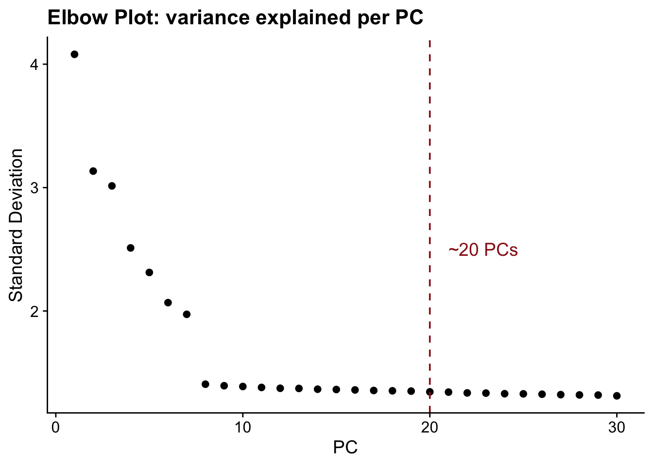
The elbow is where adding more PCs explains little additional variance.

Use this to set dims in FindNeighbors and RunUMAP.

ElbowPlot(sobj_filt, ndims = 30) +
  geom_vline(xintercept = 20, linetype = "dashed", color = "#991b1b") +
  annotate("text", x = 21, y = 2.5, label = "~20 PCs", hjust = 0,
           color = "#991b1b") +
  ggtitle("Elbow Plot: variance explained per PC")

TipQUESTION 4.4

How would you choose the number of PCs in a real dataset where the elbow plot does not have a sharp knee?

TipANSWER

Combine four signals: (1) cumulative variance explained, target 70-90%; (2) JackStraw permutation test, select PCs significant at chosen alpha; (3) clustering stability across dims (rerun FindClusters at dims=10, 15, 20, 25 and compute ARI between partitions); (4) biological coherence: do all expected populations separate? Report the choice and the sensitivity analysis, not a magic number.

LIVE DEMO:

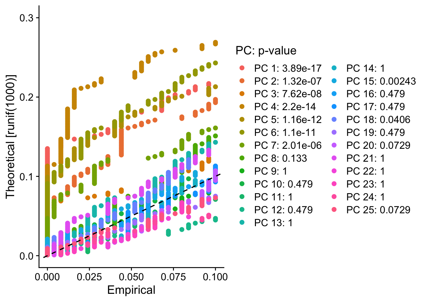
# JackStraw is slow on full data; usable on subsamples for the same conclusion
sobj_filt <- JackStraw(sobj_filt, num.replicate = 50, dims = 25, verbose = FALSE)
sobj_filt <- ScoreJackStraw(sobj_filt, dims = 1:25)
JackStrawPlot(sobj_filt, dims = 1:25)

Warning: Removed 10928 rows containing missing values or values outside the scale range
(`geom_point()`).

PLOT / OUTPUT: JackStrawPlot: PCs above the diagonal are significant

4.7.5 Step 4.4a - Sanity check: did HVG and PCA do what you asked?

• Silent failure A. FindVariableFeatures(nfeatures = 2000) on a 500-gene panel returns 500 without any warning. The HVG analysis was a no-op.

n_features  <- nrow(sobj_filt[["RNA"]])
n_hvg_asked <- 2000
n_hvg_got   <- length(VariableFeatures(sobj_filt))
cat("Features in assay  :", n_features, "\n")

Features in assay  : 500 

cat("HVG requested      :", n_hvg_asked, "\n")

HVG requested      : 2000 

cat("HVG returned       :", n_hvg_got, "\n")

HVG returned       : 500 

if (n_hvg_got < n_hvg_asked) {
  cat(">> nfeatures > total features. HVG is the full panel; the call",
      "selected nothing.\n")
}

>> nfeatures > total features. HVG is the full panel; the call selected nothing.

• Silent failure B. RunPCA returns the number of PCs you ask for, even when only a fraction carry signal. Inspect tail variance to spot dead PCs.

pca_sdev <- sobj_filt@reductions$pca@stdev
pca_var  <- pca_sdev ^ 2
cat("\nVariance explained by last 5 PCs (out of", length(pca_var), "):\n")

Variance explained by last 5 PCs (out of 30 ):

print(round(tail(pca_var / sum(pca_var) * 100, 5), 3))

[1] 1.804 1.795 1.789 1.785 1.769

cat("If the tail is below ~0.5 percent each, those PCs are mostly noise.\n")

If the tail is below ~0.5 percent each, those PCs are mostly noise.

TipQUESTION 4.4a

How many PCs carry more than 1 percent of total variance?

The line below computes it; use the result as a lower bound for dims= later.

n_pcs_above_1pct <- sum((pca_var / sum(pca_var)) > 0.01)
cat("\nNumber of PCs with > 1% variance explained:", n_pcs_above_1pct, "\n")

Number of PCs with > 1% variance explained: 30 

cat("Recommended lower bound for dims=: 1:", n_pcs_above_1pct, sep = "", "\n")

Recommended lower bound for dims=: 1:30

cat("(The elbow plot above gave ~20; this floor confirms or contradicts it.)\n")

(The elbow plot above gave ~20; this floor confirms or contradicts it.)

TipANSWER

Computed in the script. Typically 10-15 PCs carry >1% variance in this dataset; the elbow gives roughly the same number. If they disagree by more than a factor of 2, either the elbow is being misread or the dataset has unusual variance structure.

LIVE DEMO:

pca_var <- sobj_filt@reductions$pca@stdev^2
pct <- pca_var / sum(pca_var) * 100
sum(pct > 1)

[1] 30

plot(pct, type="b", xlab="PC", ylab="% variance")

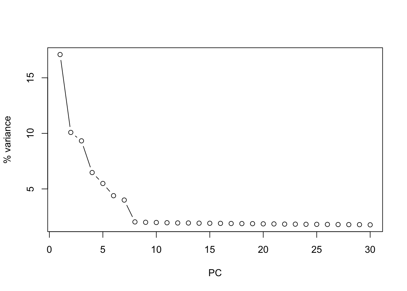
PLOT / OUTPUT: Variance-per-PC scatter; flattening point is the floor for dims

4.7.6 Step 4.4b - Decide whether to integrate (Harmony)

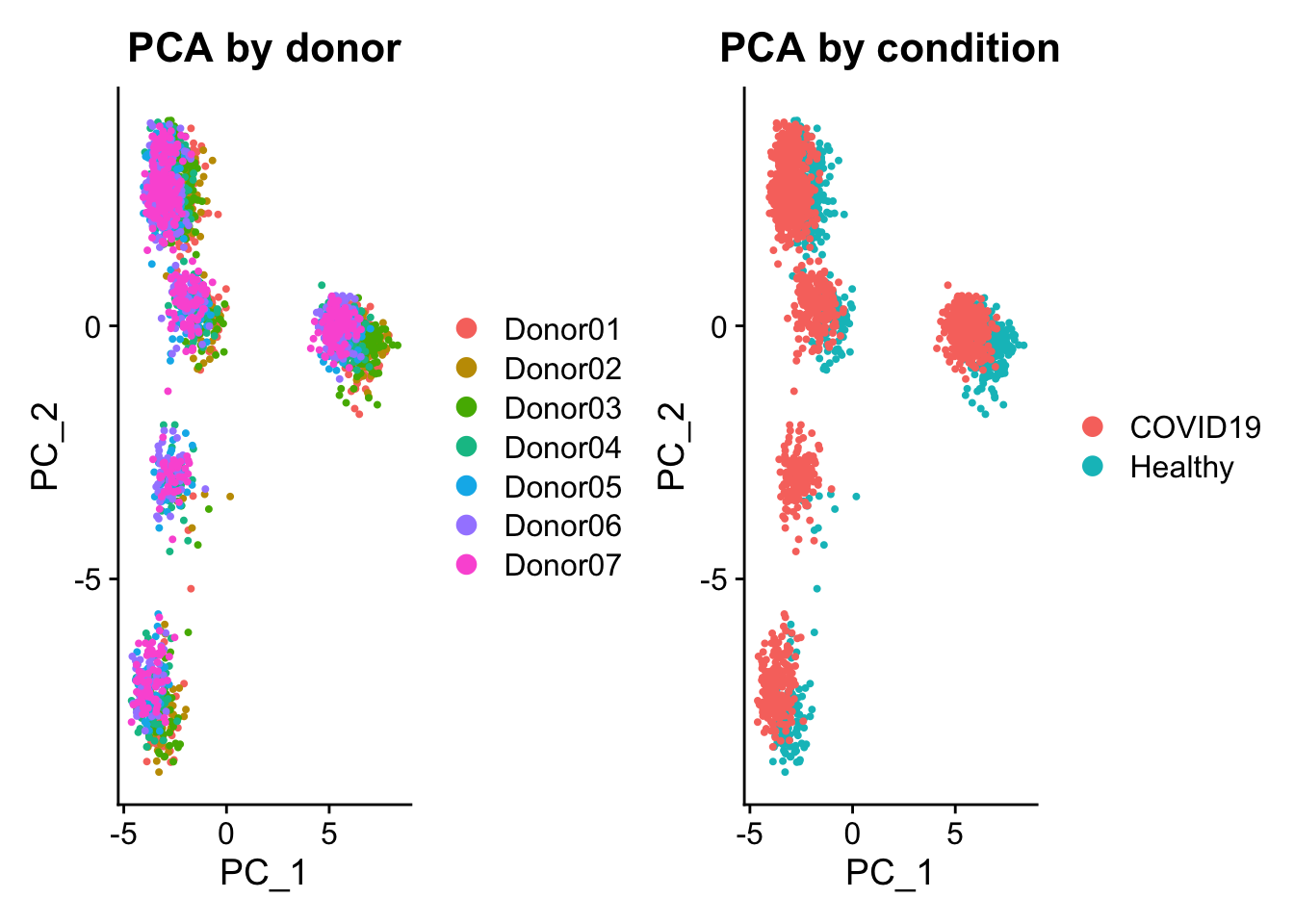
Before clustering, ask: do donors separate on the PCA? If yes, the UMAP will be donor-dominated, not biology-dominated, and clustering will encode batch.

p_pca_donor <- DimPlot(sobj_filt, reduction = "pca", group.by = "donor_id") +
  ggtitle("PCA by donor")
p_pca_cond  <- DimPlot(sobj_filt, reduction = "pca", group.by = "condition") +
  ggtitle("PCA by condition")
p_pca_donor | p_pca_cond

• Quick R^2 diagnostic: how much of PC1 and PC2 is explained by donor?

pc_coords <- Embeddings(sobj_filt, reduction = "pca")[, 1:2]
for (pc in 1:2) {
  fit <- summary(lm(pc_coords[, pc] ~ sobj_filt$donor_id))
  cat(sprintf("PC%d ~ donor_id R^2: %.3f\n", pc, fit$r.squared))
}

PC1 ~ donor_id R^2: 0.065
PC2 ~ donor_id R^2: 0.007

TipTip

Decision rule of thumb: - R^2 < 0.10 : donor effect minimal, no integration needed - R^2 0.10 to 0.30: borderline, consider integration if cell types are mixed across donors - R^2 > 0.30 : donor dominates, integration recommended

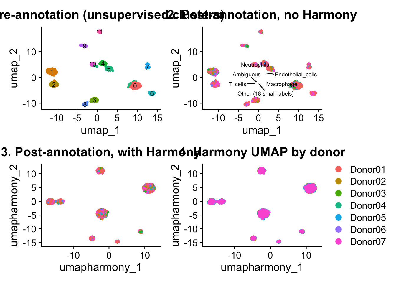
In this dataset the donor effect is borderline-to-low, so clustering and annotation through Block 5 (Section 4.8) proceed on the plain PCA/UMAP without Harmony.

Step 5.4e (Section 4.8.9) runs Harmony anyway. Once cell types are annotated, to build a side-by-side comparison panel: seeing that Harmony barely changes the layout on data you already trust is what makes you confident reading the same comparison on a new dataset where you do not yet know the answer.

Reference syntax (current harmony package, Seurat object method):

library(harmony)
# NOT RUN
sobj_harm <- RunHarmony(sobj_filt, group.by.vars = "donor_id",
                          reduction      = "pca",
                           reduction.save = "harmony",
                           verbose        = FALSE)
   DimPlot(sobj_harm, reduction = "harmony", group.by = "donor_id") +
     ggtitle("After Harmony (donor)")

In downstream FindNeighbors / RunUMAP, switch reduction = "pca" to reduction = "harmony" (dims stays the same; Harmony returns the same dimensionality as the input reduction).

TipQUESTION 4.4b

At what donor R^2 would you switch to Harmony in your own data? The block above already printed the R^2 for PC1 and PC2; apply this rule directly:

r2_pc1 <- summary(lm(pc_coords[, 1] ~ sobj_filt$donor_id))$r.squared
verdict <- if (r2_pc1 < 0.10) {
  "NO integration needed"
} else if (r2_pc1 < 0.30) {
  "BORDERLINE: integrate only if cell types are also separated by donor"
} else {
  "INTEGRATE (Harmony or similar)"
}
cat(sprintf("\nDecision for this dataset: R^2(PC1)= %.3f -> %s\n", r2_pc1, verdict))

Decision for this dataset: R^2(PC1)= 0.065 -> NO integration needed

cat("\nTrade-off of integration:\n")

Trade-off of integration:

cat("  Pro: removes technical donor variance; cell types pool across donors.\n")

  Pro: removes technical donor variance; cell types pool across donors.

cat("  Con: may remove TRUE biological inter-donor variance (e.g., one donor\n")

  Con: may remove TRUE biological inter-donor variance (e.g., one donor

cat("       genuinely lacks a cell type). Always cross-check post-integration\n")

       genuinely lacks a cell type). Always cross-check post-integration

cat("       that cell type proportions per donor remain plausible.\n")

       that cell type proportions per donor remain plausible.

TipANSWER

Thresholds (in the script): R^2 < 0.10 = no integration; 0.10-0.30 = borderline, integrate only if cell types are also separated by donor; >0.30 = integrate. Trade-off: integration removes technical donor variance so cell types pool across donors. It also removes TRUE biological inter-donor variance: if one donor genuinely lacks a cell type, integration may merge their cells with cells from other donors that DO have it, hiding the difference. After integrating, always check that per-donor cell type proportions remain plausible. This dataset’s R^2 falls in the low-to-borderline range, so clustering and annotation proceed without Harmony through Block 5 (Section 4.8). Step 5.4e (Section 4.8.9) runs Harmony anyway and Step 5.4f (Section 4.8.10) builds a 4-panel comparison so students see directly whether integration would have changed anything, rather than taking the R^2 threshold on faith.

LIVE DEMO:

pc_coords <- Embeddings(sobj_filt, "pca")[, 1:5]
sapply(1:5, function(i)
  summary(lm(pc_coords[, i] ~ sobj_filt$donor_id))$r.squared)

[1] 0.064676642 0.007479984 0.042866818 0.793805724 0.035593229

PLOT / OUTPUT: DimPlot(sobj_filt, reduction='pca', group.by='donor_id') side by side with group.by='condition'; see also the 4-panel comparison in Step 5.4f (Section 4.8.10).

4.7.7 Step 4.4c - Spot the bug

Read the code below carefully. Two things are wrong. Find both before running anything.

sobj_filt <- FindNeighbors(sobj_filt, dims = 0:20, verbose = FALSE)
sobj_filt <- RunUMAP(sobj_filt, dims = c(1, 2, 3, 5, 7, 11, 13))

Your answer:

REVEAL:

1. dims = 0:20 includes PC 0, which does not exist. PCA indexing starts at 1. FindNeighbors will silently drop the 0 or error depending on the Seurat version. Always use 1:N.
2. dims passed as a non-contiguous vector skips intermediate PCs. UMAP will run but the result represents only the 7 selected dimensions, not the structure captured by the elbow. Always use a contiguous range starting from 1.

4.7.8 Step 4.5 - FindNeighbors: a common dimension mismatch

RunPCA was called with npcs = 30. Passing dims = 1:50 to FindNeighbors asks for 50 PCs that do not exist.

# >>> DELIBERATE ERROR - read the message, then continue. <<<
try({
  # npcs=30 was used in RunPCA. What happens if we request 50 dims?
  sobj_filt <- FindNeighbors(sobj_filt, dims = 1:50, verbose = FALSE)
})

Error in FindNeighbors.Seurat(sobj_filt, dims = 1:50, verbose = FALSE) : 
  More dimensions specified in dims than have been computed

The error occurs because the PCA object contains only 30 components. - dims = 1:50 requests components that do not exist. - Common cause: npcs in RunPCA is changed but downstream calls are not updated.

sobj_filt <- FindNeighbors(sobj_filt, dims = 1:20, verbose = FALSE)

4.7.9 Step 4.6 - Resolution sensitivity and final clustering

How much does the clustering change between resolution 0.2 and 1.2?

res_values <- c(0.2, 0.5, 1.2)
n_clusters <- sapply(res_values, function(r) {
  tmp <- FindClusters(sobj_filt, resolution = r, verbose = FALSE)
  length(unique(tmp$seurat_clusters))
})

cat("Resolution vs number of clusters:\n")

Resolution vs number of clusters:

for (i in seq_along(res_values)) {
  cat("  resolution =", res_values[i], "->", n_clusters[i], "clusters\n")
}

  resolution = 0.2 -> 12 clusters
  resolution = 0.5 -> 12 clusters
  resolution = 1.2 -> 12 clusters

cat("\nUsing resolution = 0.5 for the rest of the analysis.\n")

Using resolution = 0.5 for the rest of the analysis.

sobj_filt <- FindClusters(sobj_filt, resolution = 0.5, verbose = FALSE)
cat("Clusters found:", length(unique(sobj_filt$seurat_clusters)), "\n")

Clusters found: 12 

print(table(sobj_filt$seurat_clusters))

  0   1   2   3   4   5   6   7   8   9  10  11 
527 460 347 221 198 197 165 135 118 116 107  82 

TipQUESTION 4.6

Lower resolution gives fewer, larger clusters; higher resolution gives more, smaller ones. Neither is intrinsically right.

• What evidence do you use to defend a chosen resolution?

TipANSWER

Three things: (1) biological coherence: each cluster has a distinguishable marker profile, defensible against the literature; (2) stability across nearby resolutions: clusters should not fragment dramatically on a small perturbation; ARI between resolutions 0.4 and 0.6 should be high; (3) downstream sanity: cluster count matches expectations for the tissue (PBMC at 3,000 cells: 8-14 clusters is reasonable; 25 is too many; 4 is too few). Show a clustree-style visualization across a resolution sweep and report which resolution and why.

LIVE DEMO:

for (r in c(0.3, 0.5, 0.8, 1.2)) {
  sobj_filt <- FindClusters(sobj_filt, resolution = r, verbose = FALSE)
  cat(sprintf("res=%.1f -> %d clusters\n", r, length(unique(Idents(sobj_filt)))))
}

res=0.3 -> 12 clusters
res=0.5 -> 12 clusters
res=0.8 -> 12 clusters
res=1.2 -> 12 clusters

PLOT / OUTPUT: If clustree is installed: clustree(sobj_filt, prefix=‘RNA_snn_res.’)

4.7.10 Step 4.7 - UMAP visualization

Three questions to answer immediately after generating the UMAP:

1. Do cells cluster by biology or by donor? (batch effect check)
2. Do canonical marker genes map to expected clusters?
3. Does condition (Healthy vs COVID-19) show any spatial structure? set.seed(42)

• umap.method='uwot' is the current default but Seurat prints a one-time notice when not stated explicitly. Setting it silences the notice.

sobj_filt <- RunUMAP(
  sobj_filt,
  dims        = 1:20,
  umap.method = "uwot",
  metric      = "cosine",
  verbose     = FALSE
)

Warning: The default method for RunUMAP has changed from calling Python UMAP via reticulate to the R-native UWOT using the cosine metric
To use Python UMAP via reticulate, set umap.method to 'umap-learn' and metric to 'correlation'
This message will be shown once per session

p1 <- DimPlot(sobj_filt, group.by = "seurat_clusters",
              label = TRUE, label.size = 4) +
  NoLegend() + ggtitle("Clusters (resolution = 0.5)")

p2 <- DimPlot(sobj_filt, group.by = "orig.ident") +
  ggtitle("By donor: batch effect?") +
  theme(legend.text = element_text(size = 7))

p1 | p2

p_cond <- DimPlot(sobj_filt, group.by = "condition",
                  cols = c("Healthy" = "#0d7377", "COVID19" = "#991b1b"),
                  pt.size = 0.5) +
  ggtitle("Healthy vs COVID-19")

p_sev <- DimPlot(sobj_filt, group.by = "severity",
                 pt.size = 0.5) +
  ggtitle("COVID-19 severity") +
  theme(legend.text = element_text(size = 8))

p_cond | p_sev

TipQUESTION 4.7

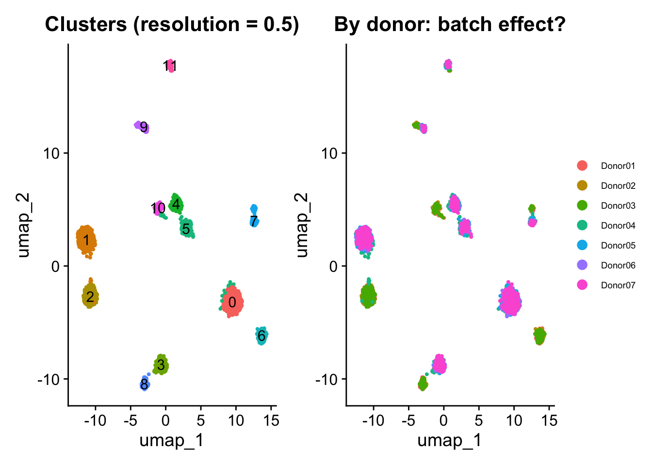
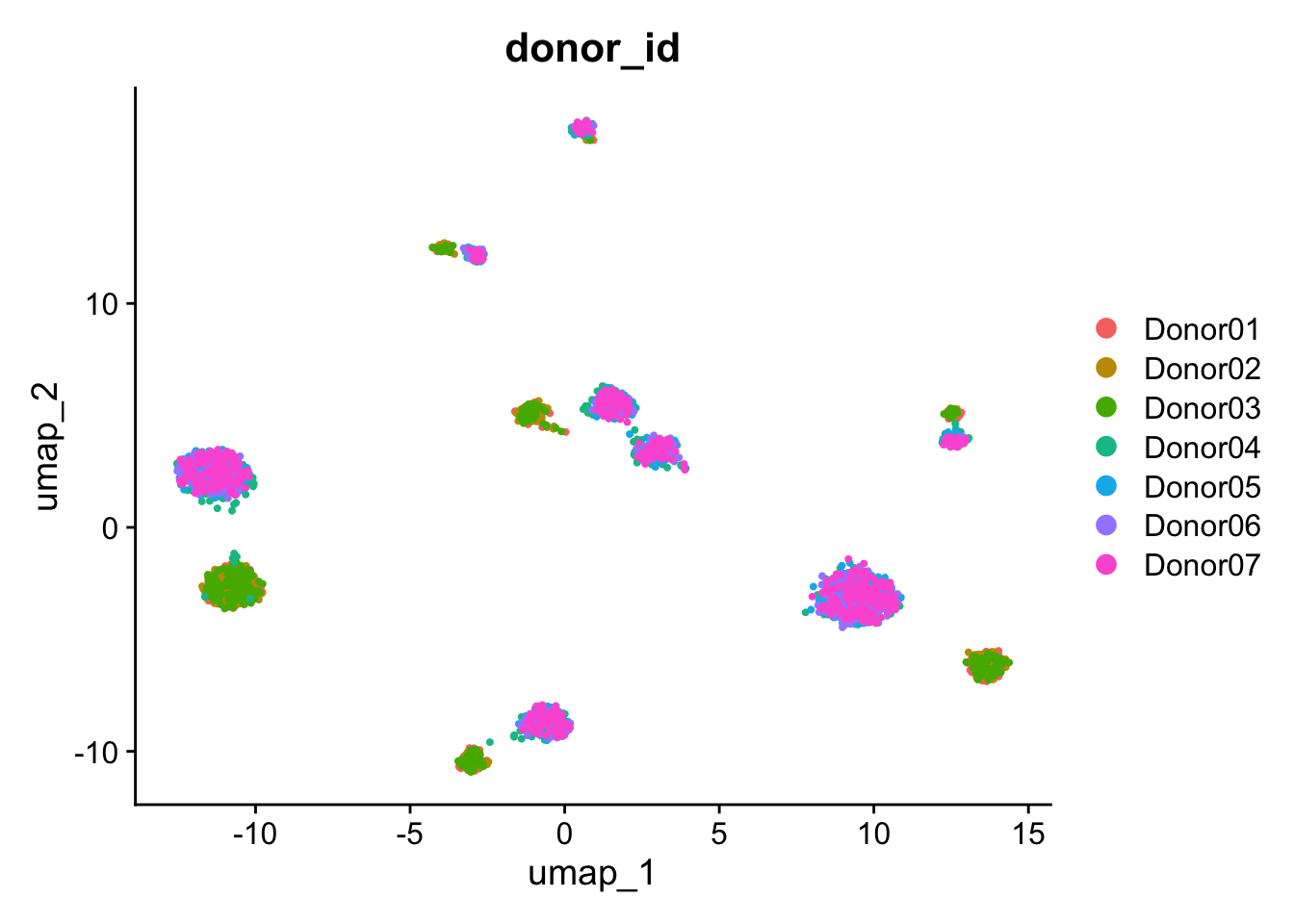
If donors visibly separate on the UMAP, is that batch effect or biology? What additional information would help you decide?

TipANSWER

Cannot tell from UMAP alone. Two checks: (1) do donors cluster within shared cell-type regions or do they form their own regions? Same cell types in same UMAP region across donors = expected biology; same cell types in DIFFERENT UMAP regions per donor = batch. Color UMAP by cell type and by donor on the same plot. (2) Compute the PC1 R^2 against donor_id (see 4.4b); if high, batch dominates the embedding.

LIVE DEMO:

DimPlot(sobj_filt, reduction="umap", group.by="donor_id") 

DimPlot(sobj_filt, reduction="umap", group.by="singler_label")

Warning: The following requested variables were not found: singler_label

Error in `[.data.frame`:
! undefined columns selected

PLOT / OUTPUT: Side-by-side UMAPs make the call obvious in most cases.

4.7.11 Step 4.8 - Canonical PBMC markers (RNA)

Match marker expression to cluster locations before formal annotation

FeaturePlot(sobj_filt,
            features   = c("CD3E", "CD19", "CD14", "NCAM1", "IL7R", "FCGR3A"),
            ncol       = 3,
            min.cutoff = "q05")

DotPlot(sobj_filt,
        features = c("CD3E", "CD4", "CD8A", "CD19", "MS4A1",
                     "CD14", "FCGR3A", "NCAM1", "PPBP"),
        group.by = "seurat_clusters") +
  RotatedAxis() +
  ggtitle("Marker expression by cluster")

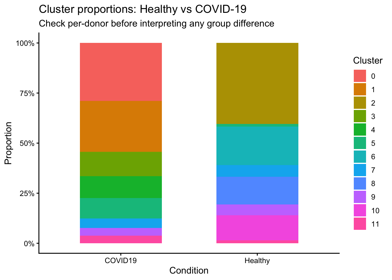
4.7.12 Step 4.9 - Cluster proportions across conditions

This is a preliminary result. It must be validated after annotation.

props <- sobj_filt@meta.data %>%
  group_by(condition, seurat_clusters) %>%
  summarise(n = n(), .groups = "drop") %>%
  group_by(condition) %>%
  mutate(prop = n / sum(n))

ggplot(props, aes(x = condition, y = prop, fill = seurat_clusters)) +
  geom_bar(stat = "identity", width = 0.6) +
  scale_y_continuous(labels = scales::percent_format()) +
  labs(title    = "Cluster proportions: Healthy vs COVID-19",
       subtitle = "Check per-donor before interpreting any group difference",
       x = "Condition", y = "Proportion", fill = "Cluster") +
  theme_classic(base_size = 12)

4.8 Block 5 - Cell type annotation (RNA-based)

Goal: assign cell type labels from a curated reference (SingleR with the Human Primary Cell Atlas), then verify the labelled object before the CITE-seq workflow begins. RNA-only annotation has known weaknesses for T cell subsets; Block 6 (Section 5.1) will revisit those with protein.

4.8.1 Step 5.1 - Run SingleR against Human Primary Cell Atlas

Option A — Standard Installation Path

👉 This workflow uses the official Human Primary Cell Atlas reference and is the recommended confirmatory approach.

cat("Loading reference (Human Primary Cell Atlas)...\n")
ref     <- celldex::HumanPrimaryCellAtlasData()
rna_mat <- LayerData(sobj_filt, assay = "RNA", layer = "data")

cat("Running SingleR...\n")
singler_res <- SingleR(
  test    = rna_mat,
  ref     = ref,
  labels  = ref$label.main,
  BPPARAM = BiocParallel::SerialParam()
)

Option B — Alternative with Pre‑saved RDS File

If installation of celldex or other dependencies fails:

1. Download the pre‑generated file Obtain singleR.rds from the provided course materials.
2. Load file in R:

library(here) # install.packages("here")

here() starts at /private/var/folders/zz/cdcfnwts145c0xjqs_c0y6mm0000gn/T/RtmppqY2dt/file177bf5943e353

singler_res <- readRDS(
  here("checkpoints", "step5.1", "singleR.rds")
)

3. Use the labels directly These labels can be integrated into your analysis pipeline as a checkpoint, allowing you to continue without installing celldex.

👉 This workflow is exploratory and ensures reproducibility even in restricted environments (e.g., macOS ARM64 or limited internet access).

cat("\nCell type distribution:\n")

Cell type distribution:

print(sort(table(singler_res$labels), decreasing = TRUE))

             T_cells             Monocyte              NK_cell 
                 786                  447                  354 
              B_cell                   DC    Endothelial_cells 
                 307                  156                  140 
         Neutrophils           Macrophage     Pre-B_cell_CD34- 
                 138                  103                   71 
    Epithelial_cells            Platelets          Gametocytes 
                  68                   49                   14 
                 CMP            Myelocyte          Hepatocytes 
                  12                   10                    8 
                 MEP              Neurons          Fibroblasts 
                   6                    6                    5 
                  BM     Pro-B_cell_CD34+                  GMP 
                   3                    3                    1 
          HSC_-G-CSF            HSC_CD34+ Neuroepithelial_cell 
                   1                    1                    1 
       Pro-Myelocyte    Tissue_stem_cells 
                   1                    1 

cat("\nLow-confidence cells (NA in pruned labels):",
    sum(is.na(singler_res$pruned.labels)), "\n")

Low-confidence cells (NA in pruned labels): 17 

4.8.2 Step 5.2 - Plotting a label before it is in the object

Forgetting to transfer SingleR’s labels into the Seurat object before calling DimPlot(group.by = "singler_label") produces an opaque error. The label only exists in the SingleR result object until you copy it over.

# >>> DELIBERATE ERROR - read the message, then continue. <<<
try({
  # singler_res is a separate object. Labels must be transferred to sobj_filt first.
  DimPlot(sobj_filt, group.by = "singler_label")
})

Warning: The following requested variables were not found: singler_label

Error in `[.data.frame`(data, , group) : undefined columns selected

singler_label does not exist in sobj_filt@meta.data yet. singler_res is a DataFrame (Bioconductor class). The labels must be explicitly added to the Seurat metadata.

sobj_filt$singler_label  <- singler_res$labels
sobj_filt$singler_pruned <- singler_res$pruned.labels

Verify

cat("singler_label in metadata:", "singler_label" %in% colnames(sobj_filt@meta.data), "\n")

singler_label in metadata: TRUE 

cat("Distribution:\n")

Distribution:

print(sort(table(sobj_filt$singler_label), decreasing = TRUE))

             T_cells             Monocyte              NK_cell 
                 782                  445                  351 
              B_cell                   DC    Endothelial_cells 
                 305                  154                  138 
         Neutrophils           Macrophage     Pre-B_cell_CD34- 
                 136                  102                   71 
    Epithelial_cells            Platelets          Gametocytes 
                  68                   49                   14 
                 CMP            Myelocyte          Hepatocytes 
                  12                   10                    8 
                 MEP              Neurons          Fibroblasts 
                   6                    6                    4 
                  BM     Pro-B_cell_CD34+                  GMP 
                   3                    3                    1 
          HSC_-G-CSF            HSC_CD34+ Neuroepithelial_cell 
                   1                    1                    1 
       Pro-Myelocyte    Tissue_stem_cells 
                   1                    1 

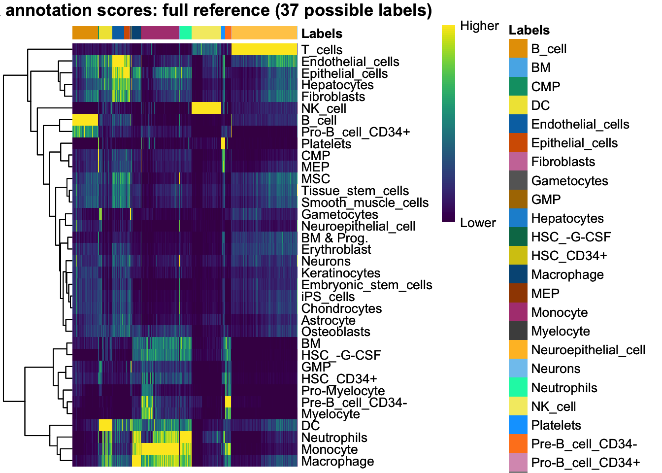
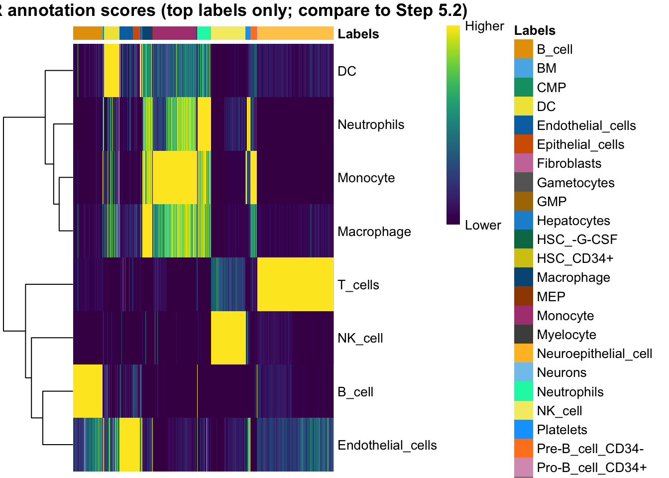
Cells with similar scores across multiple types are ambiguous. Wide spread = high confidence. Narrow spread = low confidence. plotScoreHeatmap() draws one row per possible reference label: the FULL HumanPrimaryCellAtlasData catalog, ~37 rows, regardless of how many cells were actually assigned to each. Look at this before any cleanup happens. Most of those 37 rows will show almost no signal for any cell in this dataset; that visual clutter is the evidence that motivates the consolidation in the next step.

plotScoreHeatmap(singler_res,
                 main = "SingleR annotation scores: full reference (37 possible labels)")

TipQUESTION 5.2

How many of the rows in this heatmap show any real signal (a cluster of cells with a clearly bright cell)? What does the rest of the rows tell you about how many of the labels printed above are likely noise?

TipANSWER

On this dataset, typically only 5 to 8 of the roughly 37 rows show a clear bright block: a clean separation where one column-group of cells lights up brightly for that row and stays dark for the rest. Those rows correspond to the real cell populations actually present in PBMC: T cells, B cells, monocytes, NK cells, and a few others. The remaining rows are close to uniformly dim across every cell. A dim row does not mean SingleR made an error; it means no cell in this dataset scored highly against that reference label, which is expected for labels like Hepatocytes or Neurons in a blood sample. The practical reading: if a label’s row in this heatmap never lights up brightly anywhere, any cell assigned that label by the raw classifier is suspect, and that is exactly why so many distinct values appeared in the ‘Cell type distribution’ printed in Step 5.2 (Section 4.8.2). The dim rows are the visual evidence that motivates collapsing low-frequency labels together in Step 5.2b (Section 4.8.3), rather than trusting all of them as equally real populations.

LIVE DEMO:

Count distinct labels with at least one confidently assigned cell:

label_tab <- sort(table(sobj_filt$singler_label), decreasing = TRUE)
print(label_tab)

             T_cells             Monocyte              NK_cell 
                 782                  445                  351 
              B_cell                   DC    Endothelial_cells 
                 305                  154                  138 
         Neutrophils           Macrophage     Pre-B_cell_CD34- 
                 136                  102                   71 
    Epithelial_cells            Platelets          Gametocytes 
                  68                   49                   14 
                 CMP            Myelocyte          Hepatocytes 
                  12                   10                    8 
                 MEP              Neurons          Fibroblasts 
                   6                    6                    4 
                  BM     Pro-B_cell_CD34+                  GMP 
                   3                    3                    1 
          HSC_-G-CSF            HSC_CD34+ Neuroepithelial_cell 
                   1                    1                    1 
       Pro-Myelocyte    Tissue_stem_cells 
                   1                    1 

Compare to how many rows visually ‘light up’ in the heatmap above.

PLOT / OUTPUT: The full plotScoreHeatmap from Step 5.2 (Section 4.8.2) (37 rows); count how many show a bright block versus uniform dimness.

4.8.3 Step 5.2b - Consolidate to top-N labels and check distribution plausibility

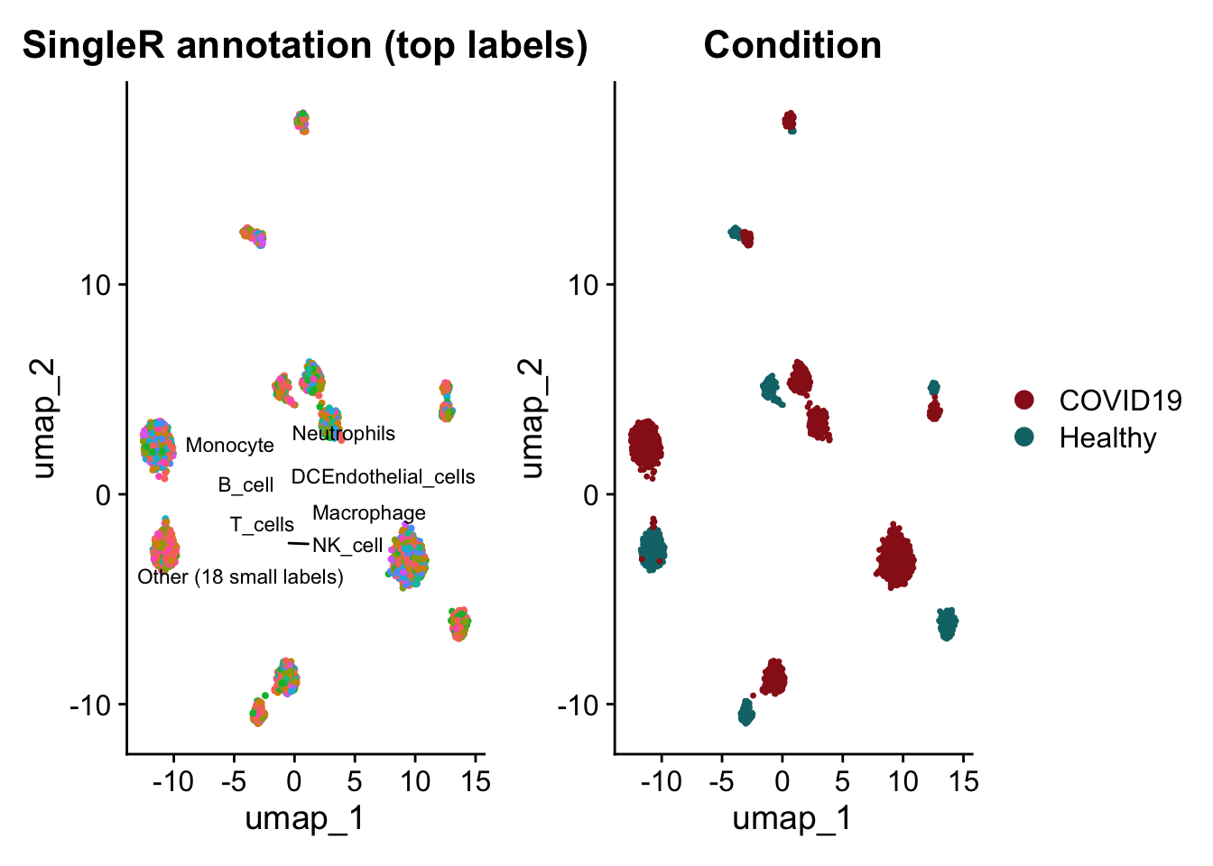
HumanPrimaryCellAtlasData covers dozens of cell types across many tissues. On a 500-gene PBMC panel it typically returns 20+ distinct labels, most supported by only a handful of cells (low-confidence noise, not real populations). Plotting all of them produces an unreadable legend and defeats the purpose of every downstream comparison.

singler_label (full detail) is kept untouched in the metadata for cases where the exact label matters. singler_label_top collapses every label outside the top N most frequent into “Other (n small labels)” and is what every plot from here on uses by default. The same pass that builds the consolidation also checks whether the underlying distribution looks like a real PBMC annotation, since both questions come from the same table.

What this step decides, and what it does not: this is a count-based decision about which CATEGORIES are worth their own color in a plot. It never looks at a single gene or a single cell’s expression. A cell labeled “T_cell” stays “T_cell” here regardless of whether it actually expresses any T cell marker; the only thing that changes is whether that label gets its own slot in the legend or gets folded into “Other” because too few cells share it.

Step 5.4a (Section 4.8.6), later, asks a different question on top of this one: given a label that survived this filter, does the individual cell carrying it actually show the expression evidence that label implies? That is a per-cell, marker-based check, not a per-label, count-based one.

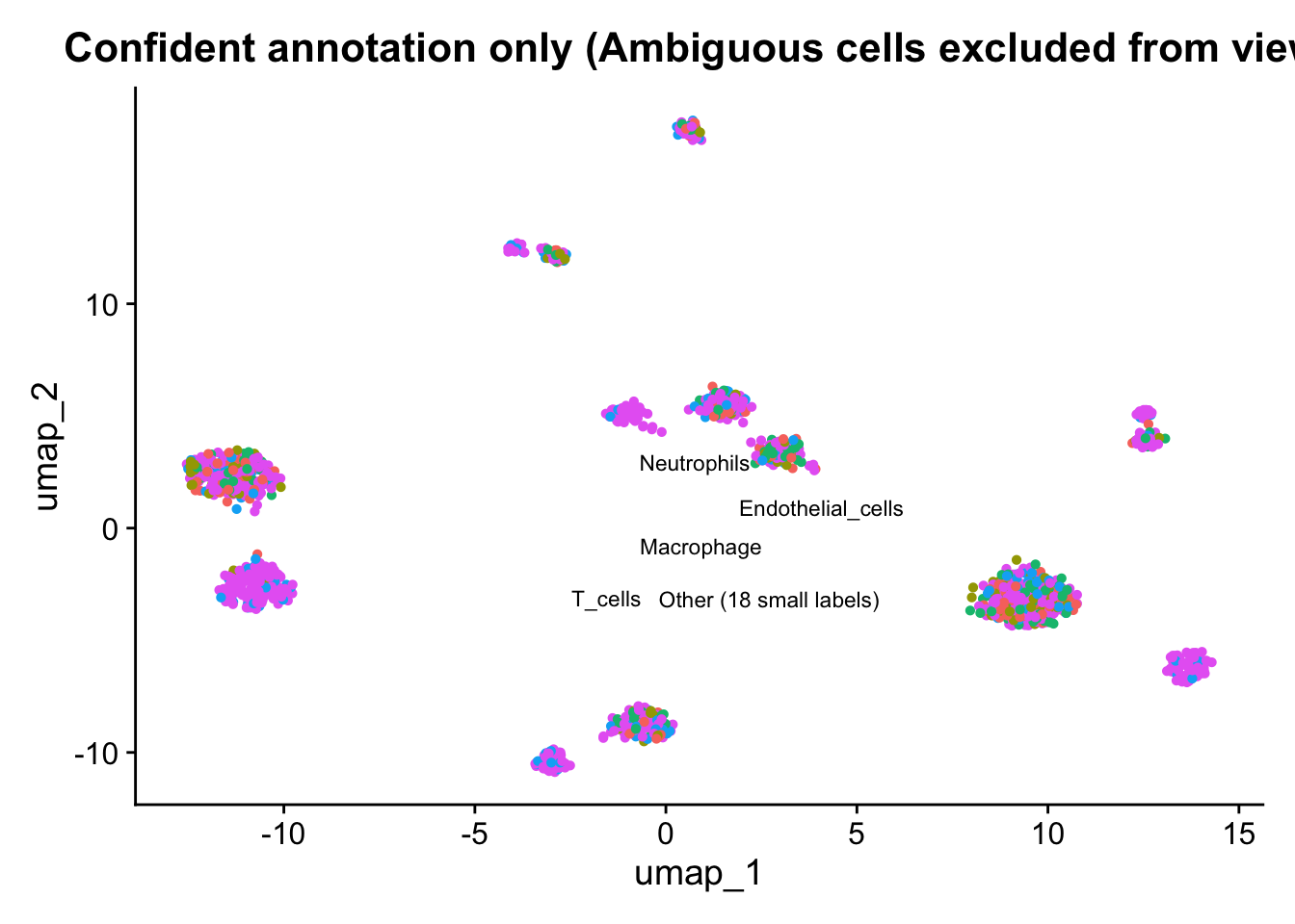
Step 5.4c (Section 4.8.7) then builds singler_label_clean directly from singler_label_top, adding only the cells that failed the Step 5.4a (Section 4.8.6) marker check as a new “Ambiguous” category. The two steps are not redundant: this one decides what to show, Step 5.4a/5.4c (Section 4.8.6 / Section 4.8.7) decides who to trust within what is shown.

TOP_N_LABELS <- 8

label_tab <- sort(table(sobj_filt$singler_label), decreasing = TRUE)
top_labels <- names(label_tab)[seq_len(min(TOP_N_LABELS, length(label_tab)))]
n_collapsed <- length(label_tab) - length(top_labels)

sobj_filt$singler_label_top <- ifelse(
  sobj_filt$singler_label %in% top_labels,
  sobj_filt$singler_label,
  sprintf("Other (%d small labels)", n_collapsed)
)
sobj_filt$singler_label_top <- factor(
  sobj_filt$singler_label_top,
  levels = c(top_labels, sprintf("Other (%d small labels)", n_collapsed))
)

cat(sprintf("Kept top %d labels, collapsed %d smaller labels into 'Other':\n",
            length(top_labels), n_collapsed))

Kept top 8 labels, collapsed 18 smaller labels into 'Other':

print(table(sobj_filt$singler_label_top))

                T_cells                Monocyte                 NK_cell 
                    782                     445                     351 
                 B_cell                      DC       Endothelial_cells 
                    305                     154                     138 
            Neutrophils              Macrophage Other (18 small labels) 
                    136                     102                     260 

Sanity rules of thumb for PBMC, checked against the full (uncollapsed) label table:

• Expect 3 to 7 dominant labels (T cells, B cells, monocytes, NK cells, DC)
• One label > 80% of all cells: suspicious (annotation collapse)
• More than 15 distinct labels in 3,000 cells: reference too granular
• Any single non-immune label > 5% (e.g. hepatocytes, fibroblasts): wrong reference

n_labels <- length(label_tab)
top_prop <- max(label_tab) / sum(label_tab)
cat(sprintf("\nDistinct labels (full table): %d  |  Dominant label proportion: %.1f%%\n",
            n_labels, top_prop * 100))

Distinct labels (full table): 26  |  Dominant label proportion: 29.3%

if (n_labels > 15) cat(">> Many distinct labels. Reference may be too granular for PBMC.\n")

>> Many distinct labels. Reference may be too granular for PBMC.

if (top_prop > 0.80) cat(">> One label dominates. Check whether reference matches the tissue.\n")

TipQUESTION 5.2b

Look at the labels collapsed into “Other” (the rows of label_tab beyond rank 8). Are any of them biologically plausible for PBMC (e.g. “Platelets”, “DC”) or all implausible (e.g. “Hepatocytes”, “Neurons”)? What would you do differently if a plausible label got collapsed away?

TipANSWER

On this dataset, HumanPrimaryCellAtlasData typically returns 20+ labels for a 500-gene PBMC panel. Most of what falls outside the top 8 is biologically implausible for blood (Hepatocytes, Fibroblasts, Endothelial_cells, Neurons, Gametocytes, Astrocytes) and reflects low-confidence noise from a reference that covers many tissues, not a PBMC-specific signal. A few collapsed labels CAN be biologically plausible but rare in this cohort (Platelets, DC, Pro-B_cell subsets) - those are real minority populations, just small ones. The top-N consolidation is a visualization aid, not a correction to the annotation itself: singler_label (uncollapsed) is preserved in the metadata for exactly this reason. If a plausible rare population matters to your analysis (e.g. you are specifically studying platelets or DCs), raise TOP_N_LABELS, or keep using singler_label directly for that one analysis instead of singler_label_top.

LIVE DEMO:

Inspect what fell into “Other”:

label_tab <- sort(table(sobj_filt$singler_label), decreasing = TRUE)
print(label_tab[-(1:8)])

    Pre-B_cell_CD34-     Epithelial_cells            Platelets 
                  71                   68                   49 
         Gametocytes                  CMP            Myelocyte 
                  14                   12                   10 
         Hepatocytes                  MEP              Neurons 
                   8                    6                    6 
         Fibroblasts                   BM     Pro-B_cell_CD34+ 
                   4                    3                    3 
                 GMP           HSC_-G-CSF            HSC_CD34+ 
                   1                    1                    1 
Neuroepithelial_cell        Pro-Myelocyte    Tissue_stem_cells 
                   1                    1                    1 

Raise TOP_N_LABELS if a plausible rare population is being collapsed:

TOP_N_LABELS <- 12

PLOT / OUTPUT: Console output (table of collapsed labels and their counts).

4.8.4 Step 5.3 - Annotated UMAP and the cleaned-up heatmap

p_ann <- DimPlot(sobj_filt, group.by = "singler_label_top",
                 label = TRUE, label.size = 3, repel = TRUE) +
  ggtitle("SingleR annotation (top labels)") + NoLegend()

p_cond <- DimPlot(sobj_filt, group.by = "condition",
                  cols = c("Healthy" = "#0d7377", "COVID19" = "#991b1b"),
                  pt.size = 0.4) +
  ggtitle("Condition")

p_ann | p_cond

Same heatmap as Step 5.2 (Section 4.8.2), restricted to the labels that survived the top-N consolidation. Compare directly against the full 37-row version shown earlier: this is what “readable” looks like once the labels that carried no real signal have been set aside.

cat("Labels passed to labels.use:\n")

Labels passed to labels.use:

print(top_labels)

[1] "T_cells"           "Monocyte"          "NK_cell"          
[4] "B_cell"            "DC"                "Endothelial_cells"
[7] "Neutrophils"       "Macrophage"       

heatmap_result <- tryCatch({
  plotScoreHeatmap(singler_res,
                   labels.use = top_labels,
                   main = "SingleR annotation scores (top labels only; compare to Step 5.2)")
  "filtered"
}, error = function(e) {
  message("labels.use raised an error in this SingleR version: ", conditionMessage(e))
  message("Falling back to the full heatmap.")
  plotScoreHeatmap(singler_res,
                   main = "SingleR annotation scores (wider spread = more confident)")
  "full (fallback)"
})

cat("Heatmap actually drawn:", heatmap_result, "\n")

Heatmap actually drawn: filtered 

cat("If this says 'full (fallback)', the plot above is identical to Step 5.2\n")

If this says 'full (fallback)', the plot above is identical to Step 5.2

cat("by design: that is the fallback path, not the filtered version.\n")

by design: that is the fallback path, not the filtered version.

4.8.5 Step 5.4 - Verify the annotated object

Compare the object now with its state in Section 4.4 (Block 1) before moving to the CITE-seq workflow.

cat("Object after RNA workflow + annotation:\n")

Object after RNA workflow + annotation:

print(sobj_filt)

An object of class Seurat 
524 features across 2673 samples within 2 assays 
Active assay: RNA (500 features, 500 variable features)
 3 layers present: counts, data, scale.data
 1 other assay present: ADT
 2 dimensional reductions calculated: pca, umap

cat("\nReductions :", paste(SafeReductions(sobj_filt), collapse = ", "), "\n")

Reductions : pca, umap 

cat("Assays     :", paste(SafeAssays(sobj_filt), collapse = ", "), "\n")

Assays     : RNA, ADT 

cat("New metadata columns vs pre-QC:\n")

New metadata columns vs pre-QC:

print(setdiff(colnames(sobj_filt@meta.data), colnames(sobj@meta.data)))

[1] "scDblFinder.class" "scDblFinder.score" "is_dbl"           
[4] "RNA_snn_res.0.3"   "RNA_snn_res.0.8"   "RNA_snn_res.1.2"  
[7] "singler_label"     "singler_pruned"    "singler_label_top"

TipQUESTION 5.4

• Which slots are still empty / unchanged in the ADT assay?
• What does that tell you about what Block 6 (Section 5.1) needs to do first?

TipANSWER

ADT still has only the counts layer. No data layer (no normalization), no scale.data, no var.features, no reductions referencing ADT. Block 6 (Section 5.1) must build the ADT side from scratch:normalize (CLR margin=2), then either use it directly for plots and gating (no scale.data needed) or run RunPCA on the ADT counts before WNN.

LIVE DEMO:

Layers(sobj_filt[["ADT"]])

[1] "counts" "data"  

Reductions(sobj_filt)

[1] "pca"  "umap"

PLOT / OUTPUT: Console output

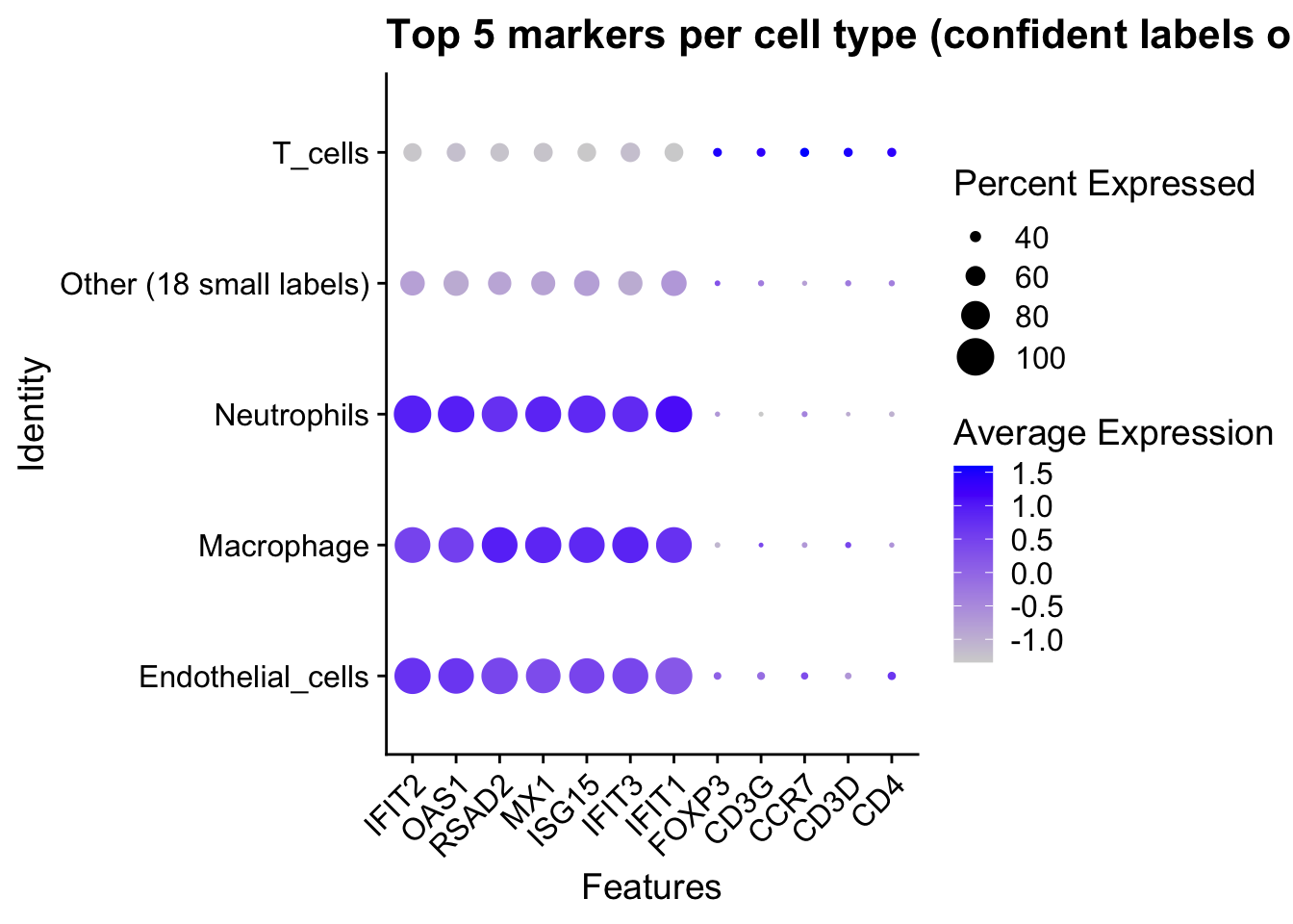
4.8.6 Step 5.4a - Canonical-marker validation per cell type

Before trusting an annotation, verify the canonical RNA marker of each major lineage is detected in a reasonable fraction of cells assigned to that lineage. The label-distribution sanity check already ran in Step 5.2b (Section 4.8.3), right after the labels were consolidated; this step is a different kind of check, on the per-marker evidence rather than the label counts.

Step 5.2b (Section 4.8.3) asked “how many cells share this label, and is that count plausible for PBMC?” That is a question about labels as categories: it never inspected a single gene. This step asks a different question: “for a cell that carries this label, does its RNA actually show the marker that label implies?” That is a per-cell, expression-based check, run independently of how common or rare the label was. A label can pass the Step 5.2b (Section 4.8.3) frequency check (common enough to keep its own category) and still fail this one (most cells carrying it do not express the expected marker), which is exactly what the detection-rate table below is built to catch. The output of this step (detection_rates) feeds Step 5.4c (Section 4.8.7), which builds singler_label_clean from singler_label_top and adds “Ambiguous” only for the cells that failed this marker check, on top of the categories Step 5.2b (Section 4.8.3) already decided were worth keeping.

Map SingleR label patterns to canonical markers

check_markers <- list(
  "T_cell|T cell" = c("CD3E", "CD3D"),
  "B_cell|B cell" = c("CD79A", "MS4A1"),
  "Monocyte"      = c("CD14", "LYZ"),
  "NK"            = c("NKG7", "GNLY"),
  "DC|Dendritic"  = c("FCER1A")
)

cat(sprintf("\n%-25s %-10s %-12s %s\n", "Label", "Marker", "Cells (n)", "Detection rate"))

Label                     Marker     Cells (n)    Detection rate

cat(sprintf("%-25s %-10s %-12s %s\n",   "-----", "------", "---------", "--------------"))

-----                     ------     ---------    --------------

for (lbl in unique(sobj_filt$singler_label)) {
  for (lbl_pat in names(check_markers)) {
    if (grepl(lbl_pat, lbl, ignore.case = TRUE)) {
      cell_mask <- sobj_filt$singler_label == lbl
      n_cells   <- sum(cell_mask)
      for (mk in check_markers[[lbl_pat]]) {
        if (mk %in% rownames(sobj_filt[["RNA"]])) {
          rna_vec <- FetchData(sobj_filt, vars = mk)[cell_mask, 1]
          rate    <- mean(rna_vec > 0) * 100
          flag    <- if (rate < 25) "LOW (dropout or wrong label)" else "ok"
          cat(sprintf("%-25s %-10s %-12d %.1f%% %s\n",
                      substr(lbl, 1, 25), mk, n_cells, rate, flag))
        }
      }
    }
  }
}

DC                        FCER1A     154          8.4% LOW (dropout or wrong label)
B_cell                    CD79A      305          15.7% LOW (dropout or wrong label)
B_cell                    MS4A1      305          17.4% LOW (dropout or wrong label)
Monocyte                  CD14       445          25.8% ok
Monocyte                  LYZ        445          24.7% LOW (dropout or wrong label)
T_cells                   CD3E       782          35.4% ok
T_cells                   CD3D       782          35.3% ok
Pre-B_cell_CD34-          CD79A      71           11.3% LOW (dropout or wrong label)
Pre-B_cell_CD34-          MS4A1      71           11.3% LOW (dropout or wrong label)
NK_cell                   NKG7       351          16.8% LOW (dropout or wrong label)
NK_cell                   GNLY       351          16.0% LOW (dropout or wrong label)
Pro-B_cell_CD34+          CD79A      3            0.0% LOW (dropout or wrong label)
Pro-B_cell_CD34+          MS4A1      3            0.0% LOW (dropout or wrong label)

TipQUESTION 5.4a

which annotated cell type has the lowest detection rate of its canonical marker? The code below finds it explicitly.

detection_rates <- data.frame(label = character(0), marker = character(0),
                              rate = numeric(0), stringsAsFactors = FALSE)
for (lbl in unique(sobj_filt$singler_label)) {
  for (lbl_pat in names(check_markers)) {
    if (grepl(lbl_pat, lbl, ignore.case = TRUE)) {
      cell_mask <- sobj_filt$singler_label == lbl
      for (mk in check_markers[[lbl_pat]]) {
        if (mk %in% rownames(sobj_filt[["RNA"]])) {
          rna_vec <- FetchData(sobj_filt, vars = mk)[cell_mask, 1]
          detection_rates <- rbind(detection_rates,
            data.frame(label = lbl, marker = mk,
                       rate = mean(rna_vec > 0) * 100,
                       stringsAsFactors = FALSE))
        }
      }
    }
  }
}
if (nrow(detection_rates) > 0) {
  worst <- detection_rates[which.min(detection_rates$rate), ]
  cat(sprintf("\nLowest detection: %s expressing %s at %.1f%%\n",
              worst$label, worst$marker, worst$rate))
  cat("\nDecision rule:\n")
  cat("  rate >= 50%  -> annotation consistent with RNA (no action)\n")
  cat("  rate 25-50%  -> dropout likely (ADT in Block 6 should rescue)\n")
  cat("  rate < 25%   -> suspect misannotation; cross-check with ADT now\n")
}

Lowest detection: Pro-B_cell_CD34+ expressing CD79A at 0.0%

Decision rule:
  rate >= 50%  -> annotation consistent with RNA (no action)
  rate 25-50%  -> dropout likely (ADT in Block 6 should rescue)
  rate < 25%   -> suspect misannotation; cross-check with ADT now

TipANSWER

Computed in the script. The lowest rate usually appears for a T-cell label expressing CD3E or CD3D; CD3E RNA dropout in PBMC is often 30-50%, so detection rates between 25-50% indicate dropout (recoverable in Block 6 (Section 5.1) via ADT CD3). A detection rate below 25% for any marker is more likely misannotation. Decision thresholds: >=50% ok; 25-50% dropout-explained, verify with ADT; <25% suspect, revisit annotation.

LIVE DEMO:

lbl_mask <- sobj_filt$singler_label == "T_cells"
mean(FetchData(sobj_filt, "CD3E")[lbl_mask, 1] > 0) * 100

[1] 35.42199

PLOT / OUTPUT: Console output

4.8.7 Step 5.4c - Mark inconsistent labels as Ambiguous

Cells whose canonical marker detection rate fell below 25% in Step 5.4a (Section 4.8.6) are flagged, not deleted. singler_label_clean carries the same values as singler_label_top except those flagged cells, which become “Ambiguous”. Every prior column (singler_label, singler_label_top) stays untouched.

low_conf_labels <- character(0)
if (nrow(detection_rates) > 0) {
  per_label_rate  <- aggregate(rate ~ label, data = detection_rates, FUN = min)
  low_conf_labels <- per_label_rate$label[per_label_rate$rate < 25]
}

sobj_filt$singler_label_clean <- as.character(sobj_filt$singler_label_top)
ambiguous_mask <- sobj_filt$singler_label %in% low_conf_labels
sobj_filt$singler_label_clean[ambiguous_mask] <- "Ambiguous"
sobj_filt$singler_label_clean <- factor(sobj_filt$singler_label_clean)

cat(sprintf("\nLabels flagged Ambiguous (canonical marker detection < 25%%): %d\n",
            length(low_conf_labels)))

Labels flagged Ambiguous (canonical marker detection < 25%): 6

if (length(low_conf_labels) > 0) cat(" ", paste(low_conf_labels, collapse = ", "), "\n")

  B_cell, DC, Monocyte, NK_cell, Pre-B_cell_CD34-, Pro-B_cell_CD34+ 

cat(sprintf("Cells marked Ambiguous: %d (%.1f%% of total)\n",
            sum(ambiguous_mask), 100 * mean(ambiguous_mask)))

Cells marked Ambiguous: 1329 (49.7% of total)

cat("\nFinal label distribution (singler_label_clean):\n")

Final label distribution (singler_label_clean):

print(table(sobj_filt$singler_label_clean))

              Ambiguous       Endothelial_cells              Macrophage 
                   1329                     138                     102 
            Neutrophils Other (18 small labels)                 T_cells 
                    136                     186                     782 

TipQUESTION 5.4c

Cells marked Ambiguous are still in sobj_filt and still count toward ncol(sobj_filt). Why keep them instead of deleting them outright? What would deleting them silently change about cell counts reported in every plot from here on?

TipANSWER

Keeping them preserves an honest record of what the annotation pipeline actually produced: a real fraction of cells could not be confidently typed by RNA alone, and that fraction is itself informative (it often shrinks once ADT is added in Block 6 (Section 5.1), which is the whole point of the CITE-seq workflow). Deleting them at this stage would silently shrink ncol(sobj_filt), which changes every downstream denominator: QC summaries, per-condition proportions, per-donor cell counts, and any percentage calculation would all be computed over a smaller, undocumented population. A reader of a later plot would have no way to know cells were dropped here unless the deletion were stated explicitly every time. Marking and filtering only at the plotting step (Step 5.4d, Section 4.8.8) keeps the object’s cell count meaningful throughout the rest of the script, and the Ambiguous label itself becomes a result worth reporting (for example, in Block 6 (Section 5.1) you can check whether ADT resolves some of these cells).

LIVE DEMO:

table(sobj_filt$singler_label_clean == "Ambiguous")

FALSE  TRUE 
 1344  1329 

ncol(sobj_filt)  # unchanged regardless of how many cells are Ambiguous

[1] 2673

PLOT / OUTPUT: Console output

4.8.8 Step 5.4d - Re-plot the UMAP with only confident labels

Same UMAP as Step 5.3 (Section 4.8.4), restricted to cells that were NOT flagged Ambiguous. Cells are not removed from the object; they are simply excluded from this specific plot via cells.highlight style filtering on a copy of the metadata used for plotting.

confident_cells <- colnames(sobj_filt)[sobj_filt$singler_label_clean != "Ambiguous"]
cat(sprintf("Plotting %d / %d cells (%.1f%%) with confident annotation.\n",
            length(confident_cells), ncol(sobj_filt),
            100 * length(confident_cells) / ncol(sobj_filt)))

Plotting 1344 / 2673 cells (50.3%) with confident annotation.

DimPlot(sobj_filt, cells = confident_cells,
        group.by = "singler_label_clean",
        label = TRUE, label.size = 3, repel = TRUE) +
  ggtitle("Confident annotation only (Ambiguous cells excluded from view)") +
  NoLegend()

4.8.9 Step 5.4e - Integrate with Harmony

Step 4.4b (Section 4.7.6) found the donor effect borderline-to-low in this dataset (R^2 on PC1/PC2), so integration was not required to proceed. We run it anyway here to build the comparison panel in Step 5.4f (Section 4.8.10): with vs without Harmony is a habit worth seeing on data you already understand, before relying on it on data you do not.

library(harmony)

Loading required package: Rcpp

• This is Harmony2 version 2.0.5
• Read the guide: run vignette("quickstart", package="harmony")
• Get help: Visit the website at <https://korsunskylab.github.io/harmony2/> and
report issues on <https://github.com/immunogenomics/harmony/issues>

sobj_filt <- RunHarmony(
  sobj_filt,
  group.by.vars  = "donor_id",
  reduction      = "pca",
  dims.use       = 1:20,
  reduction.save = "harmony",
  verbose        = FALSE
)

sobj_filt <- RunUMAP(
  sobj_filt,
  reduction      = "harmony",
  dims           = 1:20,
  reduction.name = "umap.harmony",
  umap.method    = "uwot",
  metric         = "cosine",
  verbose        = FALSE
)

cat("Reductions now available:", paste(SafeReductions(sobj_filt), collapse = ", "), "\n")

Reductions now available: pca, umap, harmony, umap.harmony 

Step 4.4b (Section 4.7.6) computed donor R^2 on the plain PCA before any decision was made. Now that Harmony has run, compute the same R^2 on the harmonized embedding and compare directly: this is the actual gain or loss from integrating, in the same units used to make the original decision, not just a visual impression from a UMAP.

pc_coords_pca     <- Embeddings(sobj_filt, reduction = "pca")[, 1:2]
pc_coords_harmony <- Embeddings(sobj_filt, reduction = "harmony")[, 1:2]

r2_comparison <- data.frame(
  dimension = c("PC1", "PC2"),
  r2_before_harmony = sapply(1:2, function(pc)
    summary(lm(pc_coords_pca[, pc] ~ sobj_filt$donor_id))$r.squared),
  r2_after_harmony = sapply(1:2, function(pc)
    summary(lm(pc_coords_harmony[, pc] ~ sobj_filt$donor_id))$r.squared)
)
r2_comparison$change <- r2_comparison$r2_after_harmony - r2_comparison$r2_before_harmony

cat("\nDonor R^2 before vs after Harmony:\n")

Donor R^2 before vs after Harmony:

print(r2_comparison, row.names = FALSE)

 dimension r2_before_harmony r2_after_harmony      change
       PC1       0.064676642      0.029133436 -0.03554321
       PC2       0.007479984      0.003635754 -0.00384423

Interpretation: a large negative change means Harmony successfully removed donor-driven variance from that dimension. A change near zero confirms the Step 4.4b (Section 4.7.6) read: there was little donor effect to remove in the first place, so integration cost real biological variance for essentially no batch-correction gain.

TipQUESTION 5.4e

Is the change in donor R^2 large or close to zero in this dataset? Does that match what the Step 4.4b (Section 4.7.6) decision predicted? If you ran this on a dataset with R^2 above 0.30, what change would you expect to see in this same table?

TipANSWER

On this dataset the donor R^2 was already low to borderline before Harmony (Step 4.4b, Section 4.7.6), so the change after Harmony should also be small: Harmony has little donor-driven variance left to remove, which is exactly what the Step 4.4b (Section 4.7.6) decision to skip integration predicted. This is the confirming case: if the change had turned out large here, it would mean the original PC1/PC2-only R^2 check missed a donor effect living in later PCs, and the decision not to integrate would have been wrong. On a dataset where the pre-Harmony R^2 was above 0.30 (donor effect dominant), the expected pattern is a large drop in R^2 after Harmony (often falling toward 0.05-0.15) on the dimensions Harmony was told to correct, paired with a visibly different cell-type layout in the comparison panel: that combination is what integration succeeding actually looks like in numbers, not just in a UMAP that looks nicer.

LIVE DEMO:

print(r2_comparison, row.names = FALSE)

 dimension r2_before_harmony r2_after_harmony      change
       PC1       0.064676642      0.029133436 -0.03554321
       PC2       0.007479984      0.003635754 -0.00384423

• A large negative ‘change’ column value means Harmony removed donor signal.
• A change near zero means there was little donor signal to remove.

PLOT / OUTPUT: The r2_comparison table; pair with the 4-panel UMAP comparison in Step 5.4f (Section 4.8.10).

4.8.10 Step 5.4f - Comparison panel: UMAP before/after annotation, with/without Harmony

Four panels answer four different questions about the same object:

1. Pre-annotation: do the unsupervised clusters look reasonable at all? 2. Post-annotation (no Harmony): does the annotation make sense on the embedding you actually used through Section 4.8 (Block 5, Section 4.8)? 3. Post-annotation, Harmony: did integration change which cells sit near which others? 4. Donor color on the Harmony UMAP: did Harmony actually mix donors together, or did it not need to (consistent with the Step 4.4b (Section 4.7.6) call)?

p1_preannot <- DimPlot(sobj_filt, reduction = "umap", group.by = "seurat_clusters",
                        label = TRUE, label.size = 3) +
  ggtitle("1. Pre-annotation (unsupervised clusters)") + NoLegend()

p2_postannot <- DimPlot(sobj_filt, reduction = "umap", group.by = "singler_label_clean",
                         label = TRUE, label.size = 2.5, repel = TRUE) +
  ggtitle("2. Post-annotation, no Harmony") + NoLegend()

p3_harmony_annot <- DimPlot(sobj_filt, reduction = "umap.harmony", group.by = "singler_label_clean",
                             label = TRUE, label.size = 2.5, repel = TRUE) +
  ggtitle("3. Post-annotation, with Harmony") + NoLegend()

p4_harmony_donor <- DimPlot(sobj_filt, reduction = "umap.harmony", group.by = "donor_id") +
  ggtitle("4. Harmony UMAP by donor")

(p1_preannot | p2_postannot) / (p3_harmony_annot | p4_harmony_donor)

TipQUESTION 5.4f

Compare panels 2 and 3. If the cell-type layout looks nearly identical before and after Harmony, what does that confirm about the Step 4.4b (Section 4.7.6) decision not to integrate? If it looks different, which panel would you trust for the rest of the analysis, and why?

TipANSWER

If panels 2 and 3 look nearly identical, that confirms the Step 4.4b (Section 4.7.6) read of the data: the donor effect on PC1/PC2 was already low (R^2 < 0.10-0.30 range), so Harmony has little work to do and converges to essentially the same cell-type layout. That is the expected, reassuring outcome here, and panel 4 (Harmony UMAP by donor) should still show donors reasonably mixed within each cell-type region, the same as before integration. If panels 2 and 3 looked clearly different instead, that would mean the PC1/PC2 R^2 from Step 4.4b (Section 4.7.6) under-estimated a donor effect living in later PCs, and the right move is to trust the Harmony-integrated panel (3) for downstream analysis, since it actively corrects for batch rather than just measuring it on two dimensions. Either way, the comparison panel is the check that validates (or overturns) an integration decision made earlier from a partial diagnostic.

LIVE DEMO:

Quantify the visual comparison instead of eyeballing it:

table(sobj_filt$singler_label_clean, useNA = "ifany")

              Ambiguous       Endothelial_cells              Macrophage 
                   1329                     138                     102 
            Neutrophils Other (18 small labels)                 T_cells 
                    136                     186                     782 

Compare cluster composition before/after Harmony using adjusted Rand index if you want a number instead of a plot:

mclust::adjustedRandIndex(cluster_labels_no_harmony, cluster_labels_harmony)

Error:
! object 'cluster_labels_no_harmony' not found

PLOT / OUTPUT: The 2x2 comparison panel itself (Step 5.4f, Section 4.8.10) is the answer; no separate plot needed.

4.8.11 Step 5.4g - Differential expression markers per annotated cell type

Explicit about what this test actually uses, since the object now carries both a plain PCA/UMAP and a Harmony-corrected PCA/UMAP from Step 5.4e (Section 4.8.9):

TipExplanation

• Assay: RNA, “data” layer (log-normalized counts from Block 4, Section 4.7).
  • Harmony only touches the PCA/UMAP embeddings (used for visualization and clustering); it never modifies the RNA expression values that FindAllMarkers reads. Running this on the harmonized object or the pre-Harmony object gives identical results, because DE testing here compares expression directly between groups of cells, not their position on any embedding.
• Grouping: singler_label_clean (Step 5.4c, Section 4.8.7), Ambiguous cells excluded. They are not a coherent biological group, so testing them as their own “cluster” would not mean anything.
• Filters: only.pos = TRUE (markers, not anti-markers), min.pct = 0.25 (expressed in at least 25% of one group), logfc.threshold = 0.5 (at least 1.4-fold change).

DefaultAssay(sobj_filt) <- "RNA"
Idents(sobj_filt) <- "singler_label_clean"

de_markers <- FindAllMarkers(
  subset(sobj_filt, idents = "Ambiguous", invert = TRUE),
  only.pos        = TRUE,
  min.pct         = 0.25,
  logfc.threshold = 0.5,
  verbose         = FALSE
)

For a (much!) faster implementation of the Wilcoxon Rank Sum Test,
(default method for FindMarkers) please install the presto package
--------------------------------------------
install.packages('devtools')
devtools::install_github('immunogenomics/presto')
--------------------------------------------
After installation of presto, Seurat will automatically use the more 
efficient implementation (no further action necessary).
This message will be shown once per session

Warning in FindMarkers.default(object = data.use, cells.1 = cells.1, cells.2 =
cells.2, : No features pass logfc.threshold threshold; returning empty
data.frame

TOP_N_MARKERS <- 5
top_markers <- de_markers %>%
  group_by(cluster) %>%
  slice_max(order_by = avg_log2FC, n = TOP_N_MARKERS) %>%
  ungroup()

cat(sprintf("Top %d markers per confident cell type:\n", TOP_N_MARKERS))

Top 5 markers per confident cell type:

print(top_markers[, c("cluster", "gene", "avg_log2FC", "pct.1", "pct.2", "p_val_adj")],
      n = nrow(top_markers))

# A tibble: 20 × 6
   cluster           gene  avg_log2FC pct.1 pct.2 p_val_adj
   <fct>             <chr>      <dbl> <dbl> <dbl>     <dbl>
 1 Endothelial_cells IFIT2      0.706 0.971 0.668  6.44e- 9
 2 Endothelial_cells OAS1       0.656 0.957 0.673  1.50e- 7
 3 Endothelial_cells RSAD2      0.569 0.978 0.663  6.39e- 6
 4 Endothelial_cells MX1        0.525 0.935 0.672  3.75e- 5
 5 Endothelial_cells ISG15      0.507 0.949 0.676  9.17e- 7
 6 Macrophage        RSAD2      0.851 0.961 0.673  2.38e-11
 7 Macrophage        MX1        0.805 0.971 0.677  2.45e- 6
 8 Macrophage        ISG15      0.682 0.961 0.683  5.42e- 7
 9 Macrophage        IFIT3      0.670 0.971 0.688  5.23e- 7
10 Macrophage        IFIT1      0.587 0.961 0.687  1.89e- 4
11 Neutrophils       MX1        0.853 0.963 0.67   6.24e-14
12 Neutrophils       IFIT2      0.851 1     0.666  6.55e-14
13 Neutrophils       OAS1       0.818 0.978 0.671  2.48e-13
14 Neutrophils       IFIT1      0.802 0.978 0.677  4.19e-14
15 Neutrophils       RSAD2      0.741 0.963 0.665  1.19e- 9
16 T_cells           FOXP3      0.754 0.347 0.283  6.50e- 1
17 T_cells           CD3G       0.665 0.345 0.283  1   e+ 0
18 T_cells           CCR7       0.557 0.353 0.281  8.39e- 1
19 T_cells           CD3D       0.546 0.353 0.279  5.88e- 1
20 T_cells           CD4        0.515 0.353 0.29   1   e+ 0

DotPlot(sobj_filt,
        features = unique(top_markers$gene),
        idents   = setdiff(levels(Idents(sobj_filt)), "Ambiguous"),
        group.by = "singler_label_clean") +
  RotatedAxis() +
  ggtitle(sprintf("Top %d markers per cell type (confident labels only)", TOP_N_MARKERS))

TipQUESTION 5.4g

Pick one cell type from the DotPlot. Does its top marker match a canonical marker you already know for that lineage (Step 1.8, Section 4.4.9)? If not, is that a red flag about the annotation, or a finding outside the canonical list that is worth investigating further?

TipANSWER

For most major lineages in this dataset the top DE marker should match a canonical gene from the Step 1.8 (Section 4.4.9) list: CD3D/CD3E for T cells, MS4A1/CD79A for B cells, CD14/LYZ for monocytes, NKG7/GNLY for NK cells. A match is reassuring: independent statistical evidence (DE testing) agrees with prior biological knowledge (canonical markers), which is the strongest form of validation available without an orthogonal assay. A mismatch is more interesting than alarming by itself: first rule out technical explanations (is the canonical gene even in the 500-gene panel? Check rownames(sobj_filt[['RNA']])), then consider whether the cluster is a known but less-textbook subtype (e.g. a Treg subset whose top marker is FOXP3 rather than generic CD3 genes) before treating it as a red flag about the annotation itself.

LIVE DEMO:

Check whether a canonical marker even exists in this 500-gene panel:

canonical_check <- c("CD3D","CD3E","MS4A1","CD79A","CD14","LYZ","NKG7","GNLY")
canonical_check[!canonical_check %in% rownames(sobj_filt[["RNA"]])]

character(0)

Then compare against the DotPlot’s top marker for the cell type in question

top_markers[top_markers$cluster == "T_cells", ]

# A tibble: 5 × 7
    p_val avg_log2FC pct.1 pct.2 p_val_adj cluster gene 
    <dbl>      <dbl> <dbl> <dbl>     <dbl> <fct>   <chr>
1 0.00130      0.754 0.347 0.283     0.650 T_cells FOXP3
2 0.00452      0.665 0.345 0.283     1     T_cells CD3G 
3 0.00168      0.557 0.353 0.281     0.839 T_cells CCR7 
4 0.00118      0.546 0.353 0.279     0.588 T_cells CD3D 
5 0.00542      0.515 0.353 0.29      1     T_cells CD4  

PLOT / OUTPUT: The DotPlot from Step 5.4g (Section 4.8.11); cross-reference visually against canonical markers.

4.8.12 Step 5.5 - Save the annotated checkpoint

saveRDS(top_markers, "checkpoints/outputs/top_markers.rds")
saveRDS(sobj_filt, "checkpoints/outputs/sobj_preprocessed.rds")

cat("Checkpoint saved: outputs/sobj_preprocessed.rds\n")

Checkpoint saved: outputs/sobj_preprocessed.rds

cat("To reload: sobj_filt <- readRDS('outputs/sobj_preprocessed.rds')\n")

To reload: sobj_filt <- readRDS('outputs/sobj_preprocessed.rds')

Look at the UMAP colored by condition. Does any cluster appear exclusively or predominantly in COVID-19 donors? Look at the DotPlot: which clusters could be monocytes based on CD14 and FCGR3A expression? After the break, we add the protein layer to test these interpretations.

Tip📌 Final Note for Users

At the end of this step, you may download the preprocessed Seurat object to continue with the next stage of the CITE‑seq analysis:

👉 This file contains the preprocessed Seurat object (sobj_preprocessed.rds) and serves as the starting point for downstream multimodal analysis. By saving and sharing this checkpoint, all users can proceed consistently without repeating earlier steps.

           used  (Mb) gc trigger   (Mb) limit (Mb) max used   (Mb)
Ncells 12097963 646.2   20895131 1116.0         NA 20895131 1116.0
Vcells 25248943 192.7   55366352  422.5      24576 55366352  422.5