5 CITE‑seq — Errors & Survival

5.1 Block 6 - CITE-seq integration (ADT + RNA)

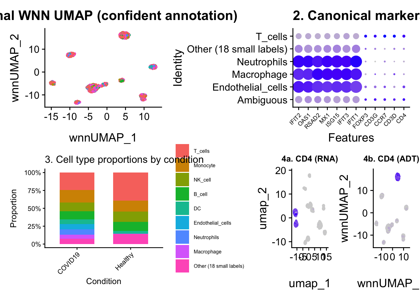
Goal: Bring the protein layer into the analysis. The RNA workflow up to Block 5 ignored ADT entirely. The CITE-seq value-add is the ability to resolve dropout, validate annotation, and weight modalities per cell.

Order of operations: inspect the ADT layer and contrast it with RNA, normalize, QC the panel, contrast RNA vs ADT for matched markers, gate, cross-check for swapped channels, build the ADT PCA, then integrate with WNN.

Load file in R:

Code

library(here) # install.packages("here")

here() starts at /private/var/folders/zz/cdcfnwts145c0xjqs_c0y6mm0000gn/T/RtmppqY2dt/file177bf5943e353

Code

sobj_filt <- readRDS(
  here("checkpoints", "outputs", "sobj_preprocessed.rds")
)
# top markers
top_markers <- readRDS(
  here("checkpoints", "outputs", "top_markers.rds")
)

Code

DefaultAssay(sobj_filt) <- "ADT"
adt_counts <- LayerData(sobj_filt, assay = "ADT", layer = "counts")

cat("ADT count matrix:\n")

ADT count matrix:

Code

cat("  Proteins (rows):", nrow(adt_counts), "\n")

  Proteins (rows): 24

Code

cat("  Cells   (cols) :", ncol(adt_counts), "\n")

  Cells   (cols) : 2673

Code

cat("  Class          :", class(adt_counts), "\n")

  Class          : dgCMatrix

Code

cat("  Layers in ADT  :", paste(SafeLayers(sobj_filt[["ADT"]]), collapse = ", "), "\n\n")

  Layers in ADT  : counts, data

Per-protein summary: scale and distribution:

Code

adt_summary <- data.frame(
  protein  = rownames(adt_counts),
  min      = apply(adt_counts, 1, min),
  median   = apply(adt_counts, 1, median),
  mean     = round(Matrix::rowMeans(adt_counts), 2),
  max      = apply(adt_counts, 1, max),
  pct_zero = round(Matrix::rowMeans(adt_counts == 0) * 100, 1)
)
cat("Per-protein distribution (first 8 proteins):\n")

Per-protein distribution (first 8 proteins):

Code

print(head(adt_summary, 8), row.names = FALSE)

 protein min median  mean max pct_zero
     CD3   0      1 15.36 168     30.9
     CD4   0      1 14.08 196     35.6
    CD8a   0      1  6.00 160     40.9
    CD14   0      1 21.64 294     32.7
    CD16   0      1  9.03 186     37.3
    CD19   0      1 10.30 209     38.4
    CD20   0      1  8.16 233     39.9
    CD25   0      1  0.80   5     45.8

Per-cell total ADT count

Code

total_adt_per_cell <- Matrix::colSums(adt_counts)
cat("\nPer-cell total ADT counts:\n")


Per-cell total ADT counts:

Code

print(round(quantile(total_adt_per_cell, c(0.05, 0.25, 0.5, 0.75, 0.95)), 0))

 5% 25% 50% 75% 95% 
 67 118 149 184 244

Code

DefaultAssay(sobj_filt) <- "RNA"

QUESTION 6.0a

An ADT protein with median ~0 but max in the high hundreds is typical bimodality (background cells vs stained cells). A protein with mean below 1 in every cell is something else. Which is which in the table above?

ANSWER

Healthy bimodal: median near 0, mean a few units higher, max in the hundreds. The protein is unstained in most cells and strongly positive in its target subset. Dead antibody pattern: mean below 1, max also low (under 10), pct_zero very high. Nothing rises above background because the antibody is non-functional. In the injected dataset, CD56 shows the dead pattern; CD3, CD4, CD8a, CD14, CD19 show the bimodal pattern. Examine the table sorted by mean to spot the anomaly.

LIVE DEMO:

Code

DefaultAssay(sobj_filt) <- "ADT"
adt <- LayerData(sobj_filt, assay="ADT", layer="counts")
qc <- data.frame(
  protein  = rownames(adt),
  median   = apply(adt, 1, median),
  mean     = round(Matrix::rowMeans(adt), 2),
  max      = apply(adt, 1, max),
  pct_zero = round(Matrix::rowMeans(adt == 0)*100, 1)
)
qc[order(qc$mean), ]

       protein median  mean max pct_zero
PD1        PD1      1  0.79   5     46.0
CD25      CD25      1  0.80   5     45.8
CD45RO  CD45RO      1  0.80   5     44.0
LAG3      LAG3      1  0.80   6     43.7
CD69      CD69      1  0.81   6     44.1
CD197    CD197      1  0.81   5     44.1
TIGIT    TIGIT      1  0.81   5     44.4
CD62L    CD62L      1  0.82   6     43.0
CD86      CD86      1  2.66 117     44.7
CD45RA  CD45RA      1  2.86  84     40.4
CD57      CD57      1  3.38  66     39.5
CD27      CD27      1  3.66 163     42.0
IgD        IgD      1  4.17  79     39.5
CD8a      CD8a      1  6.00 160     40.9
CD38      CD38      1  6.07 204     41.3
CD127    CD127      1  7.56  87     36.1
CD20      CD20      1  8.16 233     39.9
CD56      CD56      1  8.37 181     38.5
CD16      CD16      1  9.03 186     37.3
CD19      CD19      1 10.30 209     38.4
CD4        CD4      1 14.08 196     35.6
CD3        CD3      1 15.36 168     30.9
CD14      CD14      1 21.64 294     32.7
HLADR    HLADR      1 21.82 219     29.3

Code

DefaultAssay(sobj_filt) <- "RNA"

PLOT / OUTPUT:

Could also use:

Code

RidgePlot(sobj_filt, features=rownames(sobj_filt[['ADT']])[1:6], assay='ADT')

Picking joint bandwidth of 0.346

Picking joint bandwidth of 0.174

Picking joint bandwidth of 0.11

Picking joint bandwidth of 0.449

Picking joint bandwidth of 0.149

Picking joint bandwidth of 0.141

5.1.1 Step 6.0b - RNA sparsity vs ADT sparsity

Block 1 (Section 4.4) measured RNA sparsity on its own. Now that the ADT layer has been inspected too, the comparison is the point: the same cells, two assays, very different zero rates.

Code

rna_counts_b6 <- LayerData(sobj_filt, assay = "RNA", layer = "counts")
rna_sparsity  <- 1 - Matrix::nnzero(rna_counts_b6) / prod(dim(rna_counts_b6))
adt_sparsity  <- 1 - Matrix::nnzero(adt_counts)     / prod(dim(adt_counts))

cat("RNA sparsity:", round(rna_sparsity * 100, 1), "%\n")

RNA sparsity: 90.5 %

Code

cat("ADT sparsity:", round(adt_sparsity * 100, 1), "%\n")

ADT sparsity: 40.1 %

QUESTION 6.0b

Why is ADT sparsity so much lower than RNA sparsity? What does each zero mean biologically in the two modalities?

ANSWER

RNA sparsity in this 500+9-gene subset is still substantial; ADT sparsity is typically below 5%. A single mRNA molecule must be captured by an oligo-dT primer, reverse-transcribed, amplified, and sequenced. The capture and RT steps fail at a substantial rate per molecule, producing a zero where the gene was expressed. This is dropout. An ADT zero comes from antibody staining: cells are incubated with hundreds-to-thousands of antibody molecules per protein, sequencing depth for protein tags is also higher per cell. The only way to read zero is for the protein to be absent or below detection background. RNA zeros mix true absence with capture failure; ADT zeros are mostly true absence.

LIVE DEMO:

Code

rna <- LayerData(sobj_filt, assay="RNA", layer="counts")
adt <- LayerData(sobj_filt, assay="ADT", layer="counts")
mean(rna == 0) * 100        # RNA sparsity %

[1] 90.51942

Code

mean(adt == 0) * 100        # ADT sparsity %

[1] 40.0876

Code

# CD4 specifically:
sum(rna["CD4", ] == 0) / ncol(rna) * 100

[1] 67.34007

Code

sum(adt["CD4", ] == 0) / ncol(adt) * 100

[1] 35.61541

PLOT / OUTPUT: Console; histograms of per-cell zero rate also work for visual impact

5.1.2 Step 6.1 - Re-inspect the ADT layer

ADT has been sitting untouched since Block 1 (Section 4.4). Confirm its state explicitly before normalizing.

Code

DefaultAssay(sobj_filt) <- "ADT"
cat("ADT assay current state:\n")

ADT assay current state:

Code

cat("  Active assay : ADT\n")

  Active assay : ADT

Code

cat("  Proteins     :", nrow(sobj_filt[["ADT"]]), "\n")

  Proteins     : 24

Code

cat("  Cells (post-QC):", ncol(sobj_filt), "\n")

  Cells (post-QC): 2673

Code

cat("  Layers       :", paste(SafeLayers(sobj_filt[["ADT"]]), collapse = ", "), "\n")

  Layers       : counts, data

At this point we expect: counts only. No data, no scale.data. Normalization is the next step.

PUZZLE 6.1/A (ADT)

Without normalizing yet, which protein has the highest raw variance across cells? Is it a lineage marker (CD3, CD4, CD8a, CD14, CD19, CD56) or an activation marker (HLADR, CD69, CD25, PD1)?

Code

adt_counts <- LayerData(sobj_filt, assay = "ADT", layer = "counts")
adt_var <- apply(adt_counts, 1, var)
cat("\nTop 5 ADT proteins by raw-count variance:\n")


Top 5 ADT proteins by raw-count variance:

Code

print(round(sort(adt_var, decreasing = TRUE)[1:5], 1))

  CD14  HLADR    CD4   CD19    CD3 
1612.2 1174.4  857.6  743.2  681.4

ANSWER

Lineage markers usually win: CD4, CD8a, CD14, CD19, CD3 have the highest raw variance because they go from background-low in non-target cells to very high in target cells. Activation markers like CD69, HLADR, CD25 have lower variance because they are expressed at moderate levels in many cells. If an activation marker tops the list, the dataset may be enriched for activated cells, or one antibody is behaving unusually.

LIVE DEMO:

Code

adt <- LayerData(sobj_filt, assay="ADT", layer="counts")
var_per_prot <- apply(adt, 1, var)
sort(var_per_prot, decreasing = TRUE)[1:5]

     CD14     HLADR       CD4      CD19       CD3 
1612.2007 1174.4087  857.5612  743.1608  681.4481

PUZZLE 6.1/B (ADT)

How many cells are positive for BOTH CD4 and CD8a in the raw counts (> 5 counts each)? In healthy PBMC this should be near zero; anything substantial is a doublet or a contamination signal.

Code

cd4_pos <- adt_counts["CD4", ] > 5
cd8_pos <- adt_counts["CD8a", ] > 5
cat("\nADT CD4+ cells              :", sum(cd4_pos), "\n")


ADT CD4+ cells              : 582

Code

cat("ADT CD8a+ cells             :", sum(cd8_pos), "\n")

ADT CD8a+ cells             : 224

Code

cat("Double-positive (suspicious):", sum(cd4_pos & cd8_pos), "  (~0 expected)\n")

Double-positive (suspicious): 0   (~0 expected)

ANSWER

Double-positive CD4+/CD8a+ in raw ADT should be near zero in PBMC. More than 1-2% of cells: suspect doublets that scDblFinder missed, or antibody spillover. Investigate via nCount_RNA and total ADT for the suspect cells.

LIVE DEMO:

Code

cd4 <- adt["CD4", ] > 5
cd8 <- adt["CD8a", ] > 5
sum(cd4 & cd8)

[1] 0

Code

table(cd4 & cd8, sobj_filt$is_dbl)

       
        FALSE
  FALSE  2673

PLOT / OUTPUT: Console output

QUESTION 6.1

Does the double-positive count match what you expect biologically, or does it indicate doublets that survived scDblFinder? What would you do about it before annotating T cell subsets?

ANSWER

Expected near zero (under 1% of cells). True double-positive CD4+/CD8+ cells are rare in PBMC (some MAIT and gamma-delta T cells). More than 1-2% and the cells are likely doublets that scDblFinder missed (homotypic T-cell doublets). Cross-check against scDblFinder doublet class; if many double-positives are not flagged as doublets, increase the scDblFinder threshold or remove the double-positives manually before annotating T-cell subsets.

LIVE DEMO:

Code

adt <- LayerData(sobj_filt, assay="ADT", layer="counts")
cd4 <- adt["CD4", ] > 5
cd8 <- adt["CD8a", ] > 5
table(double_pos = cd4 & cd8, scDbl = sobj_filt$is_dbl)

          scDbl
double_pos FALSE
     FALSE  2673

PLOT / OUTPUT: Console table; small counts in (TRUE, FALSE) cell are the suspicious cases

5.1.3 Step 6.2 - ADT normalization (CLR, margin = 2)

CLR (Centered Log-Ratio) normalization. The margin argument sets the direction: + margin = 1: normalizes each protein across all cells (row means ~0) + margin = 2: normalizes each cell across all proteins (column means ~0)

margin = 2 is correct for CITE-seq. It removes per-cell variation in total antibody capture, analogous to library size normalization in RNA. margin = 1 runs without error but destroys biological signal. You will diagnose a real object normalized the wrong way in Block 8, Scenario 3.

Code

DefaultAssay(sobj_filt) <- "ADT"

sobj_filt <- NormalizeData(
  sobj_filt,
  normalization.method = "CLR",
  margin               = 2  # CORRECT: normalizes each cell across proteins
)

Normalizing layer: counts

Normalizing across cells

Code

adt_m2 <- LayerData(sobj_filt, layer = "data")
cat("Column means after margin=2 (per cell), expected ~0:\n")

Column means after margin=2 (per cell), expected ~0:

Code

print(round(colMeans(adt_m2)[1:8], 4))

CELL000011 CELL000021 CELL000031 CELL000041 CELL000051 CELL000061 CELL000071 
    0.5889     0.6480     0.4619     0.6050     0.5824     0.6226     0.5801 
CELL000081 
    0.5344

Code

cat("\nRow means (per protein), should NOT be ~0 (biological variation preserved):\n")


Row means (per protein), should NOT be ~0 (biological variation preserved):

Code

print(round(rowMeans(adt_m2), 4))

   CD3    CD4   CD8a   CD14   CD16   CD19   CD20   CD25   CD27   CD38 CD45RA 
1.0745 0.8865 0.5040 1.1483 0.7338 0.7100 0.5979 0.2592 0.4233 0.4623 0.4362 
CD45RO   CD56   CD57  CD62L   CD69   CD86  CD127  CD197    PD1  TIGIT   LAG3 
0.2617 0.6312 0.5058 0.2677 0.2645 0.3738 0.7574 0.2646 0.2555 0.2631 0.2601 
   IgD  HLADR 
0.5157 1.2983

Code

DefaultAssay(sobj_filt) <- "RNA"
cat("\nADT normalized correctly.\n")


ADT normalized correctly.

QUESTION 6.2

Why is the row mean a useful diagnostic? What would the row means look like if margin had been set to 1?

ANSWER

After CLR with margin=2 (per cell across proteins), column means are ~0 by construction (each cell’s protein values were centered). Row means (per protein across cells) carry the biological signal of which proteins are abundant and should NOT be near zero. They reflect dataset-wide protein abundance differences. If margin=1 was used instead (per protein across cells), row means would be near zero. That is the wrong-margin fingerprint. Cenario 3 of Block 7 contains exactly this failure.

LIVE DEMO:

Code

sobj_filt <- NormalizeData(sobj_filt, assay="ADT",
                           normalization.method="CLR", margin=2)

Normalizing layer: counts

Normalizing across cells

Code

d <- LayerData(sobj_filt, assay="ADT", layer="data")
round(rowMeans(d), 3)

   CD3    CD4   CD8a   CD14   CD16   CD19   CD20   CD25   CD27   CD38 CD45RA 
 1.074  0.887  0.504  1.148  0.734  0.710  0.598  0.259  0.423  0.462  0.436 
CD45RO   CD56   CD57  CD62L   CD69   CD86  CD127  CD197    PD1  TIGIT   LAG3 
 0.262  0.631  0.506  0.268  0.264  0.374  0.757  0.265  0.256  0.263  0.260 
   IgD  HLADR 
 0.516  1.298

Code

round(colMeans(d), 3)[1:5]

CELL000011 CELL000021 CELL000031 CELL000041 CELL000051 
     0.589      0.648      0.462      0.605      0.582

PLOT / OUTPUT: Console output; row means != 0, col means ~ 0.

5.1.4 Step 6.3 - ADT panel QC: detect dead / failed antibodies

A failed conjugation or degraded antibody produces a “dead channel”: the protein reads near zero in every cell, with almost no variance. It does not error. If you gate or annotate on a dead channel, you silently lose a whole population.

Code

DefaultAssay(sobj_filt) <- "ADT"
adt_counts <- LayerData(sobj_filt, layer = "counts")

panel_qc <- data.frame(
  protein   = rownames(adt_counts),
  median    = round(apply(adt_counts, 1, median), 2),
  mean      = round(Matrix::rowMeans(adt_counts), 2),
  pct_zero  = round(Matrix::rowMeans(adt_counts == 0) * 100, 1),
  max       = apply(adt_counts, 1, max)
)
panel_qc <- panel_qc[order(panel_qc$mean), ]
cat("ADT panel QC (sorted by mean; suspicious = bottom rows):\n")

ADT panel QC (sorted by mean; suspicious = bottom rows):

Code

print(head(panel_qc, 6), row.names = FALSE)

 protein median mean pct_zero max
     PD1      1 0.79     46.0   5
    CD25      1 0.80     45.8   5
  CD45RO      1 0.80     44.0   5
    LAG3      1 0.80     43.7   6
    CD69      1 0.81     44.1   6
   CD197      1 0.81     44.1   5

Code

DefaultAssay(sobj_filt) <- "RNA"

QUESTION 6.3

One protein has near-zero counts in essentially every cell while its RNA counterpart is clearly expressed in a defined cluster. Which protein, and which cell type does it mark?

ANSWER

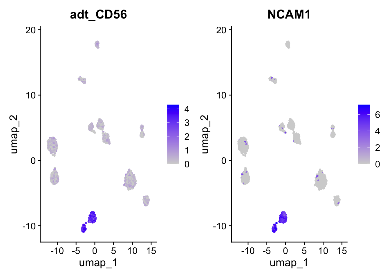
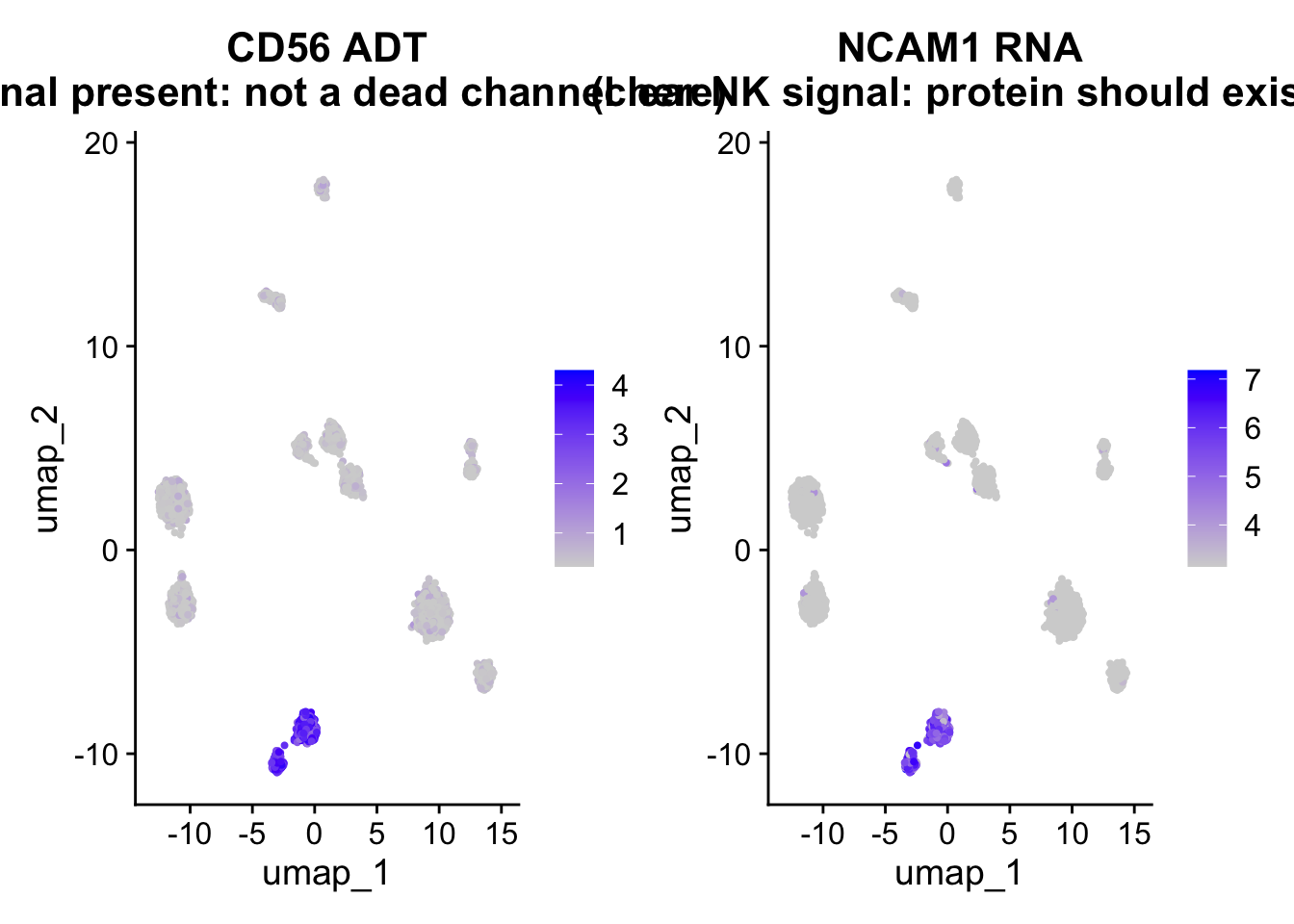
In the injected dataset: CD56 (encoded by NCAM1). CD56 marks NK cells. With CD56 ADT dead, any NK-cell annotation based on ADT alone fails. The diagnostic chunk compares CD56 ADT (near-zero) with NCAM1 RNA (clear signal in the NK cluster) and surfaces the inconsistency. Habit: always cross-check the lowest-mean ADT proteins against their RNA counterparts.

LIVE DEMO:

Code

FeaturePlot(sobj_filt, c("CD56", "NCAM1"), reduction = "umap")

Warning: Could not find CD56 in the default search locations, found in 'ADT'
assay instead

PLOT / OUTPUT: FeaturePlot panel: CD56 ADT (flat) next to NCAM1 RNA (positive in a cluster)

Compare the suspect protein (ADT) against its RNA gene side by side.

Edit suspect_adt / suspect_rna to the protein flagged above.

Code

suspect_adt <- "CD56"     # protein flagged as near-zero in panel QC
suspect_rna <- "NCAM1"    # its RNA counterpart (NK marker)

Decide the title from the actual panel_qc numbers instead of asserting a fixed claim. On the clean object this protein is healthy; on the injected object it is dead. The title should say whichever is true for the object that is actually loaded.

Code

suspect_row <- panel_qc[panel_qc$protein == suspect_adt, ]
is_dead <- nrow(suspect_row) == 1 && suspect_row$pct_zero > 90 && suspect_row$mean < 1

adt_title <- if (is_dead) {
  paste0(suspect_adt, " ADT\n(flat: likely failed antibody)")
} else {
  paste0(suspect_adt, " ADT\n(signal present: not a dead channel here)")
}

DefaultAssay(sobj_filt) <- "ADT"
p_dead <- FeaturePlot(sobj_filt, suspect_adt, min.cutoff = "q05") +
  ggtitle(adt_title)

DefaultAssay(sobj_filt) <- "RNA"
p_alive <- FeaturePlot(sobj_filt, suspect_rna, min.cutoff = "q05") +
  ggtitle(paste0(suspect_rna, " RNA\n(clear NK signal: protein should exist)"))

p_dead | p_alive

Code

DefaultAssay(sobj_filt) <- "RNA"

5.1.5 Step 6.4 - RNA vs ADT for the same marker (dropout)

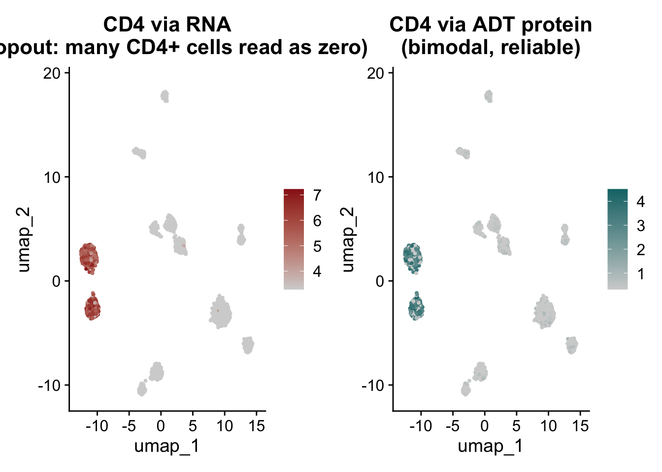
Direct comparison. CD4 mRNA reads as zero in many CD4+ T cells (dropout), while CD4 protein from ADT is bimodal across the same cells.

Code

DefaultAssay(sobj_filt) <- "RNA"
p_rna <- FeaturePlot(sobj_filt, "CD4", min.cutoff = "q05") +
  ggtitle("CD4 via RNA\n(dropout: many CD4+ cells read as zero)") +
  scale_color_gradient(low = "lightgrey", high = "#991b1b")

Scale for colour is already present.
Adding another scale for colour, which will replace the existing scale.

Code

DefaultAssay(sobj_filt) <- "ADT"
p_adt <- FeaturePlot(sobj_filt, "CD4", min.cutoff = "q05") +
  ggtitle("CD4 via ADT protein\n(bimodal, reliable)") +
  scale_color_gradient(low = "lightgrey", high = "#0d7377")

Scale for colour is already present.
Adding another scale for colour, which will replace the existing scale.

Code

p_rna | p_adt

Code

DefaultAssay(sobj_filt) <- "RNA"

5.1.6 Step 6.5 - RNA-protein correlation across all matched markers

For each ADT protein with an RNA counterpart, compute the Spearman correlation across all cells. Low correlation = high dropout in RNA.

Code

adt_rna_pairs <- list(
  CD3  = "CD3E",
  CD4  = "CD4",
  CD8a = "CD8A",
  CD14 = "CD14",
  CD19 = "CD19",
  CD56 = "NCAM1"
)

DefaultAssay(sobj_filt) <- "ADT"
adt_vals <- t(LayerData(sobj_filt, layer = "data"))
DefaultAssay(sobj_filt) <- "RNA"
rna_vals <- t(LayerData(sobj_filt, layer = "data"))

cat("Spearman correlation (RNA vs ADT) per marker:\n")

Spearman correlation (RNA vs ADT) per marker:

Code

cat(sprintf("  %-8s %s\n", "Marker", "Spearman rho"))

  Marker   Spearman rho

Code

cat(sprintf("  %-8s %s\n", "------", "------------"))

  ------   ------------

Code

for (adt_name in names(adt_rna_pairs)) {
  rna_gene <- adt_rna_pairs[[adt_name]]
  if (rna_gene %in% colnames(rna_vals) &&
      adt_name %in% colnames(adt_vals)) {
    rho <- cor(rna_vals[, rna_gene],
               adt_vals[, adt_name],
               method = "spearman")
    cat(sprintf("  %-8s %.3f\n", adt_name, rho))
  }
}

  CD3      0.753
  CD4      0.585
  CD8a     0.225
  CD14     0.727
  CD19     0.502
  CD56     0.540

Code

DefaultAssay(sobj_filt) <- "RNA"

5.1.7 Step 6.6 - Quantify dropout: ADT-positive but RNA-zero cells

For each marker, find cells that are clearly protein-positive (ADT > threshold) but have zero RNA counts. These are the cells that would be misannotated by RNA-only analysis.

Code

DefaultAssay(sobj_filt) <- "ADT"
adt_data <- LayerData(sobj_filt, layer = "data")
DefaultAssay(sobj_filt) <- "RNA"
rna_counts <- LayerData(sobj_filt, layer = "counts")

cat("Dropout analysis: cells positive by ADT but zero by RNA\n")

Dropout analysis: cells positive by ADT but zero by RNA

Code

cat(sprintf("  %-8s %-12s %-12s %s\n",
            "Marker", "ADT+ cells", "RNA==0 among ADT+", "Dropout rate"))

  Marker   ADT+ cells   RNA==0 among ADT+ Dropout rate

Code

cat(sprintf("  %-8s %-12s %-12s %s\n",
            "------", "----------", "-----------------", "------------"))

  ------   ----------   ----------------- ------------

Code

marker_pairs <- list(CD4 = "CD4", CD14 = "CD14", CD19 = "CD19")
for (adt_name in names(marker_pairs)) {
  rna_gene <- marker_pairs[[adt_name]]
  if (rna_gene %in% rownames(rna_counts) && adt_name %in% rownames(adt_data)) {
    adt_pos  <- which(adt_data[adt_name, ] > 1.0)
    rna_zero <- sum(rna_counts[rna_gene, adt_pos] == 0)
    pct      <- round(rna_zero / length(adt_pos) * 100, 1)
    cat(sprintf("  %-8s %-12d %-12d %s%%\n",
                adt_name, length(adt_pos), rna_zero, pct))
  }
}

  CD4      595          12           2%
  CD14     811          126          15.5%
  CD19     480          171          35.6%

QUESTION 6.6

For a marker with 80% dropout, what fraction of cells would be misannotated by an RNA-only workflow? Quick arithmetic:

Code

cat("\nWorked example: 80% dropout on CD4 RNA\n")


Worked example: 80% dropout on CD4 RNA

Code

cat("  Single-marker decision (CD4 RNA > 0): misses 80% of true CD4+ cells.\n")

  Single-marker decision (CD4 RNA > 0): misses 80% of true CD4+ cells.

Code

cat("  Marker panel of N independent markers (each with 80% dropout):\n")

  Marker panel of N independent markers (each with 80% dropout):

Code

cat("    P(all N drop)= 0.8^N\n")

    P(all N drop)= 0.8^N

Code

for (n in c(1, 2, 3, 5)) {
  cat(sprintf("    N = %d markers -> %.1f%% of cells still misannotated\n",
              n, 0.8^n * 100))
}

    N = 1 markers -> 80.0% of cells still misannotated
    N = 2 markers -> 64.0% of cells still misannotated
    N = 3 markers -> 51.2% of cells still misannotated
    N = 5 markers -> 32.8% of cells still misannotated

Code

cat("Rule of thumb: with 80% per-marker dropout, you need >= 3 independent\n")

Rule of thumb: with 80% per-marker dropout, you need >= 3 independent

Code

cat("markers in the panel to reduce misannotation below 50%.\n")

markers in the panel to reduce misannotation below 50%.

ANSWER

Single-marker decisions: up to 80% misannotated for cells whose RNA dropped out. The script prints the arithmetic for 1, 2, 3, 5 independent markers (each with 80% dropout): rule P(all drop) = 0.8^N. So 64%, 51%, 33% with 2, 3, 5 markers respectively. Annotation should never depend on a single marker for a high-dropout gene. ADT rescues because protein dropout is near zero.

LIVE DEMO:

Code

for (n in 1:5) cat(sprintf("N=%d -> %.1f%% still miss\n", n, 0.8^n*100))

N=1 -> 80.0% still miss
N=2 -> 64.0% still miss
N=3 -> 51.2% still miss
N=4 -> 41.0% still miss
N=5 -> 32.8% still miss

PLOT / OUTPUT: Console output

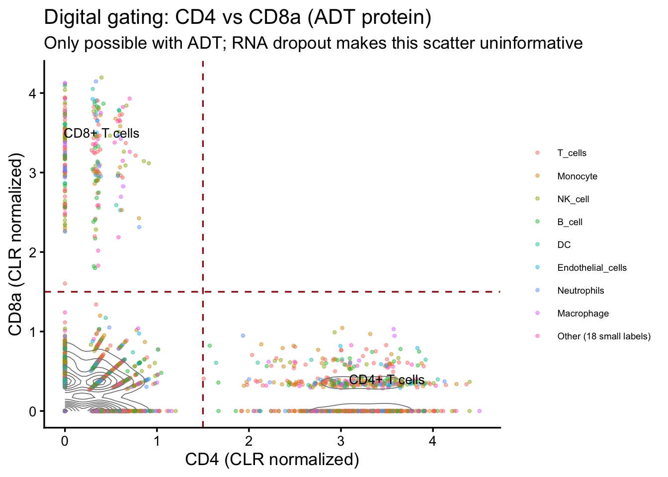
5.1.8 Step 6.7 - Digital gating

Digital gating replicates the biaxial scatter plots from flow cytometry using ADT data. It allows computational cell classification with the same logic immunologists use at the bench.

Code

DefaultAssay(sobj_filt) <- "ADT"

color_by <- if ("singler_label_top" %in% colnames(sobj_filt@meta.data)) {
  "singler_label_top"
} else {
  "cell_type"
}

gate_data <- FetchData(sobj_filt, vars = c("CD4", "CD8a", color_by))
names(gate_data)[3] <- "label"

ggplot(gate_data, aes(CD4, CD8a, color = label)) +
  geom_point(alpha = 0.4, size = 0.8) +
  geom_density_2d(color = "grey50", linewidth = 0.3) +
  geom_vline(xintercept = 1.5, linetype = "dashed", color = "#991b1b") +
  geom_hline(yintercept = 1.5, linetype = "dashed", color = "#991b1b") +
  annotate("text", x = 3.5, y = 0.4, label = "CD4+ T cells", size = 3.5) +
  annotate("text", x = 0.4, y = 3.5, label = "CD8+ T cells", size = 3.5) +
  labs(title    = "Digital gating: CD4 vs CD8a (ADT protein)",
       subtitle = "Only possible with ADT; RNA dropout makes this scatter uninformative",
       x = "CD4 (CLR normalized)", y = "CD8a (CLR normalized)",
       color = NULL) +
  theme_classic(base_size = 13) +
  theme(legend.text = element_text(size = 7))

Code

DefaultAssay(sobj_filt) <- "RNA"

5.1.9 Step 6.7b - Silent failure: DefaultAssay forgotten between calls

A function call that “works” on the wrong assay produces a silent error.

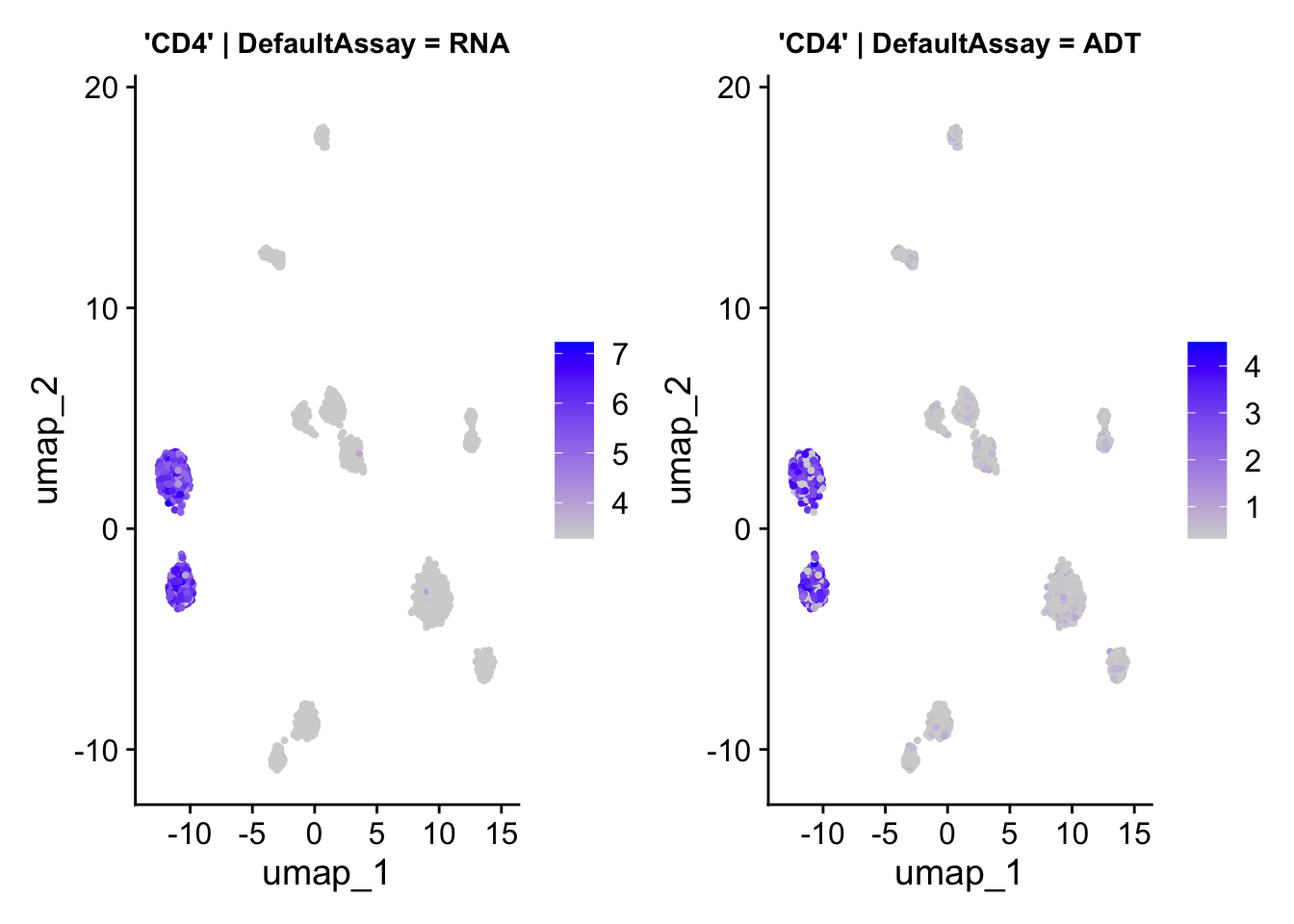
FeaturePlot("CD4") with DefaultAssay = "RNA" plots the CD4 RNA gene.
FeaturePlot("CD4") with DefaultAssay = "ADT" plots the CD4 protein.

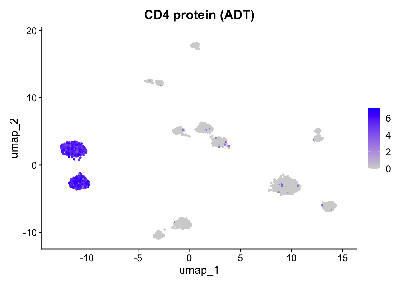
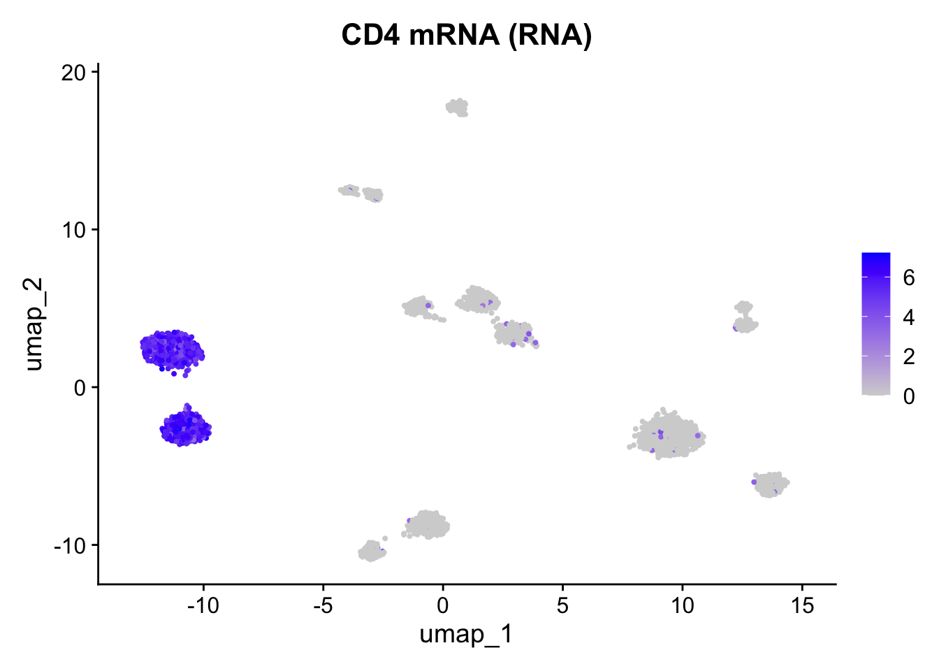
The plot RENDERS in both cases, and the two plots can look deceptively similar: min.cutoff = "q05" rescales each panel’s color gradient to its own value range, so a sparse RNA signal and a dense ADT signal both end up stretched across a similar-looking color scale. The failure is silent precisely because nothing in the rendered plot warns you which assay produced it.

Quantify the difference that the plot alone hides: what fraction of cells read exactly zero in each modality for this marker.

Code

DefaultAssay(sobj_filt) <- "RNA"
cd4_rna_zero_pct <- mean(LayerData(sobj_filt, layer = "counts")["CD4", ] == 0) * 100
DefaultAssay(sobj_filt) <- "ADT"
cd4_adt_zero_pct <- mean(LayerData(sobj_filt, layer = "counts")["CD4", ] == 0) * 100
DefaultAssay(sobj_filt) <- "RNA"

cat(sprintf("CD4 zero rate: %.1f%% of cells in RNA, %.1f%% of cells in ADT\n",
            cd4_rna_zero_pct, cd4_adt_zero_pct))

CD4 zero rate: 67.3% of cells in RNA, 35.6% of cells in ADT

Code

cat("The plots below can look similar at a glance; the zero rates above are\n")

The plots below can look similar at a glance; the zero rates above are

Code

cat("the actual difference the two assays are reporting for the same gene.\n")

the actual difference the two assays are reporting for the same gene.

Demonstrate by drawing the same call under both assays. Titles are kept short and font size is constrained, since the two plots render side by side at half width each.

Code

DefaultAssay(sobj_filt) <- "RNA"
p_as_rna <- FeaturePlot(sobj_filt, "CD4", min.cutoff = "q05") +
  ggtitle("'CD4' | DefaultAssay = RNA") +
  theme(plot.title = element_text(size = 11))

DefaultAssay(sobj_filt) <- "ADT"
p_as_adt <- FeaturePlot(sobj_filt, "CD4", min.cutoff = "q05") +
  ggtitle("'CD4' | DefaultAssay = ADT") +
  theme(plot.title = element_text(size = 11))

p_as_rna | p_as_adt

Code

DefaultAssay(sobj_filt) <- "RNA"

QUESTION 6.7b

Both plots rendered, and at a glance they can look almost the same. The zero-rate numbers printed above tell a different story. If you saved one of these plots as a figure for a paper without checking DefaultAssay first, which one would you have, and would a reader be able to tell from the figure alone that ‘CD4’ meant something different in each panel?

ANSWER

You would have whichever assay was active at the moment of the plot call, and a reader could not tell which one from the figure alone: the plot title says only ‘CD4’, the axes are identical UMAP coordinates, and min.cutoff='q05' rescales each panel’s own color gradient independently, so a sparse RNA signal and a denser ADT signal end up stretched across visually similar-looking scales. This is exactly why the zero-rate numbers matter: they show the real difference in what fraction of cells read as positive in each modality, a difference the rescaled color gradient hides. The published figure could silently show CD4 RNA when CD4 protein was intended, or vice versa, and nothing in the image itself would flag the mismatch. Habit: set DefaultAssay explicitly at the top of any plotting block, AND/OR pass the assay inside the call; better still, edit the plot title to include the assay name and consider reporting the zero rate alongside the figure so the modality difference is documented, not just visible to whoever already knows to look for it.

LIVE DEMO:

Code

DefaultAssay(sobj_filt) <- "RNA"
mean(LayerData(sobj_filt, layer="counts")["CD4", ] == 0) * 100   # RNA zero rate

[1] 67.34007

Code

DefaultAssay(sobj_filt) <- "ADT"
mean(LayerData(sobj_filt, layer="counts")["CD4", ] == 0) * 100   # ADT zero rate

[1] 35.61541

Code

DefaultAssay(sobj_filt) <- "RNA"
FeaturePlot(sobj_filt, "CD4") + ggtitle("CD4 protein (ADT)")

Code

FeaturePlot(sobj_filt, "CD4") + ggtitle("CD4 mRNA (RNA)")

PLOT / OUTPUT: Two FeaturePlots side by side, one per assay, distinct titles; the zero-rate numbers explain what the plots alone do not show.

5.1.10 Step 6.7c - Spot the bug

Read the code below. It looks correct. What is wrong?

Code

DefaultAssay(sobj_filt) <- "RNA"
adt_markers <- FindMarkers(sobj_filt, ident.1 = "CD4Tcell",
                             group.by = "cell_type",
                             min.pct  = 0.25)

For a (much!) faster implementation of the Wilcoxon Rank Sum Test,
(default method for FindMarkers) please install the presto package
--------------------------------------------
install.packages('devtools')
devtools::install_github('immunogenomics/presto')
--------------------------------------------
After installation of presto, Seurat will automatically use the more 
efficient implementation (no further action necessary).
This message will be shown once per session

Your answer:

REVEAL: the call asks for markers of CD4 T cells but DefaultAssay is RNA. It returns RNA markers, not ADT markers. The output is correct for RNA but does not answer the question “which proteins distinguish CD4 T cells”. Either set DefaultAssay = "ADT" first, or pass assay = "ADT" inside the FindMarkers call. The min.pct = 0.25 is also wrong for ADT (designed for sparse RNA); for ADT use a value like 0.5 or 0.0 with logfc.threshold.

5.1.11 Step 6.8 - When gating makes no biological sense: a swapped channel

A swapped or mislabeled channel runs perfectly. CLR normalizes it, FeaturePlot draws it, gating gates it. Nothing errors. The only signal is that the biology is impossible. The defense is to cross-check each protein against an independent label (its RNA marker).

Each protein should correlate with its own RNA gene across cells.

A canonical marker with rho near 0 is a mislabeled channel.

Code

DefaultAssay(sobj_filt) <- "ADT"
adt_d <- t(LayerData(sobj_filt, layer = "data"))
DefaultAssay(sobj_filt) <- "RNA"
rna_d <- t(LayerData(sobj_filt, layer = "data"))

check_pairs <- list(CD4 = "CD4", CD8a = "CD8A", CD19 = "CD19",
                    CD14 = "CD14", CD3 = "CD3E")

cat(sprintf("  %-6s %-12s %-10s\n", "ADT", "rho(self)", "verdict"))

  ADT    rho(self)    verdict

Code

cat(sprintf("  %-6s %-12s %-10s\n", "---", "---------", "-------"))

  ---    ---------    -------

Code

for (a in names(check_pairs)) {
  g <- check_pairs[[a]]
  if (a %in% colnames(adt_d) && g %in% colnames(rna_d)) {
    rho <- round(cor(adt_d[, a], rna_d[, g], method = "spearman"), 3)
    verdict <- if (rho < 0.05) "SUSPECT" else "ok"
    cat(sprintf("  %-6s %-12s %-10s\n", a, rho, verdict))
  }
}

  CD4    0.585        ok        
  CD8a   0.225        ok        
  CD19   0.502        ok        
  CD14   0.727        ok        
  CD3    0.753        ok

QUESTION 6.8:

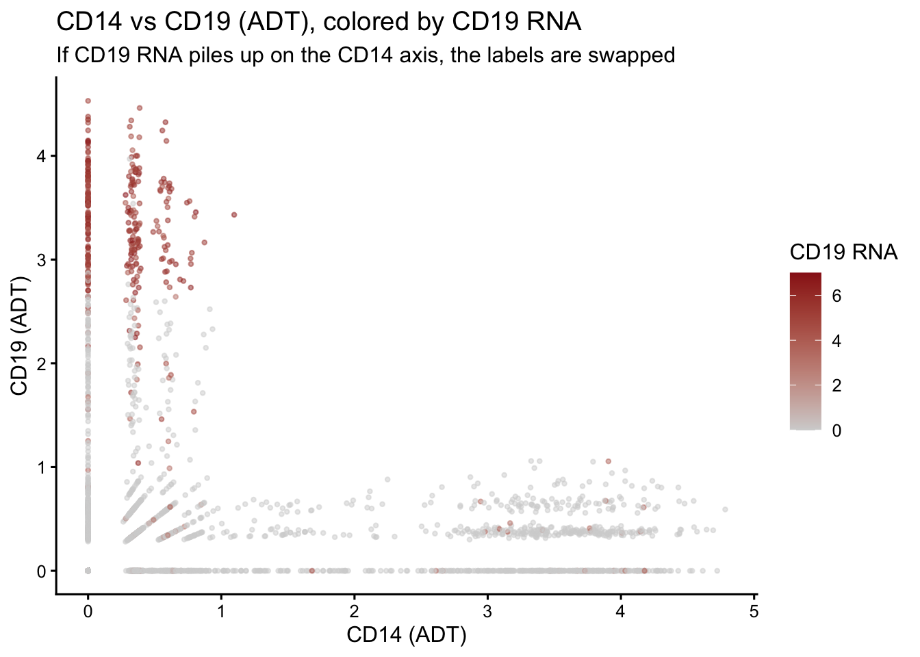
Two ADT channels show rho near 0 against their own RNA gene, while the cross pair is high. Confirm the swap with the visual below.

Code

DefaultAssay(sobj_filt) <- "ADT"
g <- FetchData(sobj_filt, vars = c("CD14", "CD19"))
DefaultAssay(sobj_filt) <- "RNA"
g$CD19_rna <- FetchData(sobj_filt, vars = "CD19")[, 1]  # B cell RNA marker

ggplot(g, aes(CD14, CD19, color = CD19_rna)) +
  geom_point(alpha = 0.5, size = 0.8) +
  scale_color_gradient(low = "lightgrey", high = "#991b1b") +
  labs(title    = "CD14 vs CD19 (ADT), colored by CD19 RNA",
       subtitle = "If CD19 RNA piles up on the CD14 axis, the labels are swapped",
       x = "CD14 (ADT)", y = "CD19 (ADT)", color = "CD19 RNA") +
  theme_classic(base_size = 12)

Code

DefaultAssay(sobj_filt) <- "RNA"

ANSWER

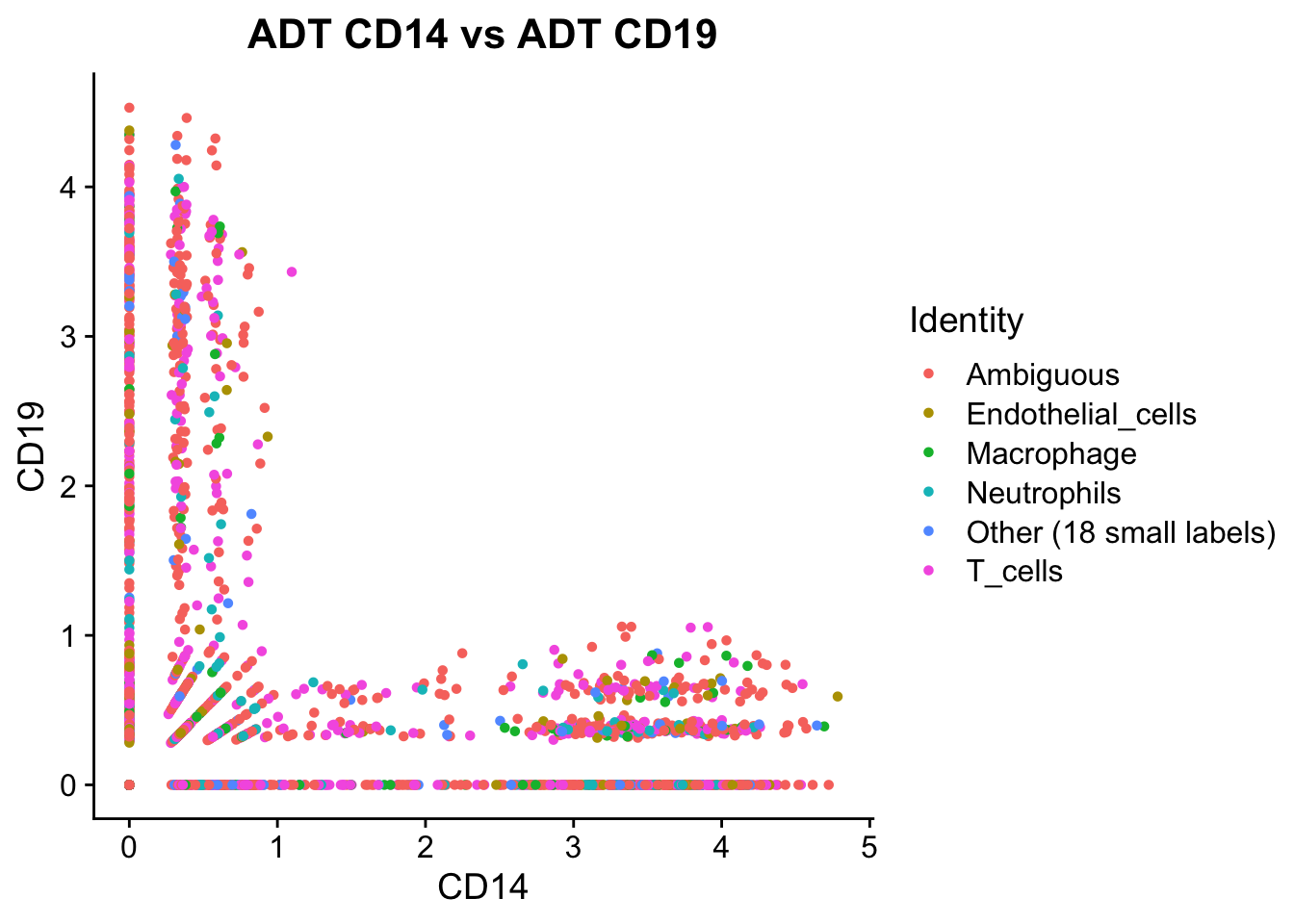
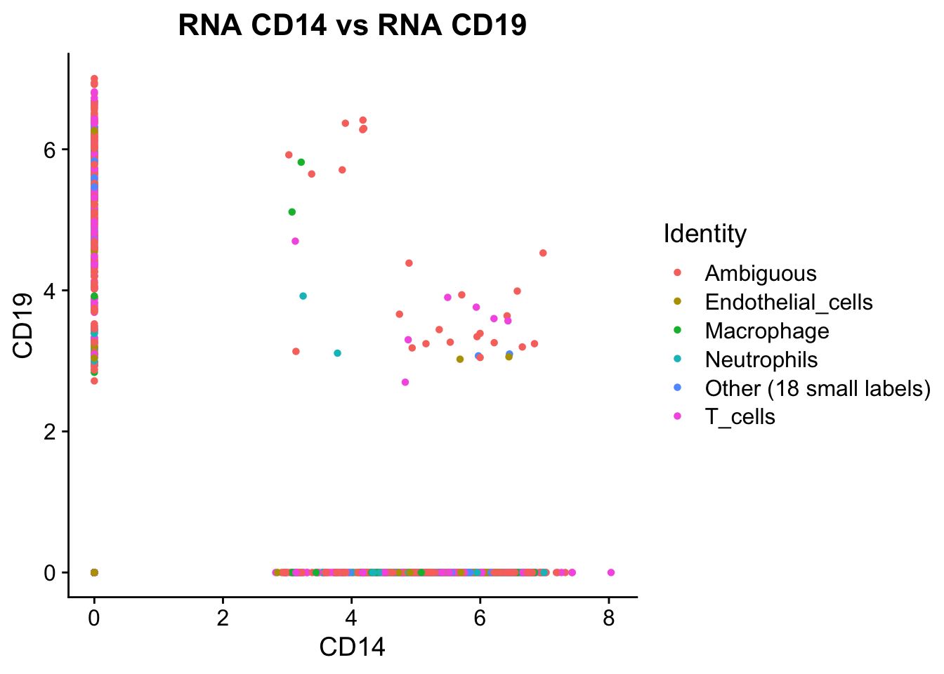
Spearman rho between each ADT protein and its RNA counterpart across cells. Healthy markers show rho 0.3-0.7. Swap fingerprint: ADT_X vs RNA_X near zero AND ADT_X vs RNA_Y high; same with X,Y reversed. In the injected dataset CD14 and CD19 ADT rownames are swapped. The fix block rebuilds the ADT assay with rownames re-swapped and re-runs CLR. Conditional, so on clean data it does nothing.

LIVE DEMO:

Code

DefaultAssay(sobj_filt) <- "ADT"
FeatureScatter(sobj_filt, "CD14", "CD19") + ggtitle("ADT CD14 vs ADT CD19")

Code

DefaultAssay(sobj_filt) <- "RNA"
FeatureScatter(sobj_filt, "CD14", "CD19") + ggtitle("RNA CD14 vs RNA CD19")

PLOT / OUTPUT: Two scatter plots side by side. Healthy: ADT and RNA scatters match. With a swap: they diverge

v5-safe: rebuild the ADT assay from its count matrix with corrected names.
Conditional: only acts if the swap is actually detected (safe on clean data).

Code

DefaultAssay(sobj_filt) <- "ADT"
adt_d <- t(LayerData(sobj_filt, layer = "data"))
rna_d <- t(LayerData(sobj_filt, assay = "RNA", layer = "data"))

swapped <- FALSE
if (all(c("CD14", "CD19") %in% colnames(adt_d))) {
  rho14 <- cor(adt_d[, "CD14"], rna_d[, "CD14"], method = "spearman")
  swapped <- is.na(rho14) || rho14 < 0.05
}

if (swapped) {
  adt_counts <- LayerData(sobj_filt, assay = "ADT", layer = "counts")
  rn  <- rownames(adt_counts)
  i14 <- which(rn == "CD14"); i19 <- which(rn == "CD19")
  rn[c(i14, i19)] <- rn[c(i19, i14)]
  rownames(adt_counts) <- rn
  # CreateAssay5Object() builds a fresh assay with only the counts layer, so
  # the [[<- replacement method warns that it differs in structure (no
  # data/scale.data layers yet) from the ADT assay it replaces. Expected and
  # harmless here; suppressWarnings() wraps the assignment itself, since the
  # notice comes from the replacement method, not from CreateAssay5Object().
  new_adt_assay <- CreateAssay5Object(counts = adt_counts)
  suppressWarnings(sobj_filt[["ADT"]] <- new_adt_assay)
  sobj_filt <- NormalizeData(sobj_filt, normalization.method = "CLR",
                             margin = 2, verbose = FALSE)
  cat("ADT labels corrected (CD14 <-> CD19) and re-normalized.\n")
} else {
  cat("No swap detected; ADT labels left unchanged.\n")
}

No swap detected; ADT labels left unchanged.

Code

# Re-check
adt_d <- t(LayerData(sobj_filt, layer = "data"))
rna_d <- t(LayerData(sobj_filt, assay = "RNA", layer = "data"))
for (a in c("CD14", "CD19")) {
  rho <- round(cor(adt_d[, a], rna_d[, a], method = "spearman"), 3)
  cat(sprintf("  %-6s rho(self) = %s\n", a, rho))
}

  CD14   rho(self) = 0.727
  CD19   rho(self) = 0.502

Code

DefaultAssay(sobj_filt) <- "RNA"

5.1.12 Step 6.9 - WNN: compute ADT PCA, then integrate

Weighted Nearest Neighbor integration learns the relative contribution of each modality per cell. Cells where RNA is informative receive more RNA weight; cells where protein is more discriminating receive more ADT weight. WNN requires a PCA per modality. RNA PCA exists from Block 4; we now build the ADT PCA.

Code

DefaultAssay(sobj_filt) <- "ADT"

adt_features <- rownames(sobj_filt[["ADT"]])  # all 24 proteins

sobj_filt <- ScaleData(
  sobj_filt,
  features = adt_features,
  verbose  = FALSE
)

With 24 proteins, requesting 20 PCs triggers a Seurat warning about computing too many singular values via truncated SVD. Two fixes both work:

1. reduce npcs to 15 (still captures the structure), or
1. pass approx = FALSE to use exact SVD.

We use (a) because 15 PCs is enough signal for 24 proteins.

Code

sobj_filt <- RunPCA(
  sobj_filt,
  features       = adt_features,
  npcs           = 15,
  reduction.name = "pca.adt",
  reduction.key  = "pcaADT_",
  verbose        = FALSE
)

Warning in svd.function(A = t(x = object), nv = npcs, ...): You're computing
too large a percentage of total singular values, use a standard svd instead.

Code

cat("Reductions now available:", paste(SafeReductions(sobj_filt), collapse = ", "), "\n")

Reductions now available: pca, umap, harmony, umap.harmony, pca.adt

Seurat expects one weight name per modality. Passing only “RNA.weight” triggers a warning that ADT.weight has been auto-assigned. Pass both explicitly to silence the notice and document the intended column names.

Code

sobj_filt <- FindMultiModalNeighbors(
  sobj_filt,
  reduction.list       = list("pca", "pca.adt"),
  dims.list            = list(1:20, 1:15),
  modality.weight.name = c("RNA.weight", "ADT.weight"),
  verbose              = FALSE
)

sobj_filt <- RunUMAP(
  sobj_filt,
  nn.name        = "weighted.nn",
  reduction.name = "wnn.umap",
  reduction.key  = "wnnUMAP_",
  verbose        = FALSE
)

Warning: The default method for RunUMAP has changed from calling Python UMAP via reticulate to the R-native UWOT using the cosine metric
To use Python UMAP via reticulate, set umap.method to 'umap-learn' and metric to 'correlation'
This message will be shown once per session

Code

DefaultAssay(sobj_filt) <- "RNA"
cat("WNN complete. New reduction: wnn.umap\n")

WNN complete. New reduction: wnn.umap

5.1.13 Step 6.10 - RNA-only UMAP vs WNN UMAP

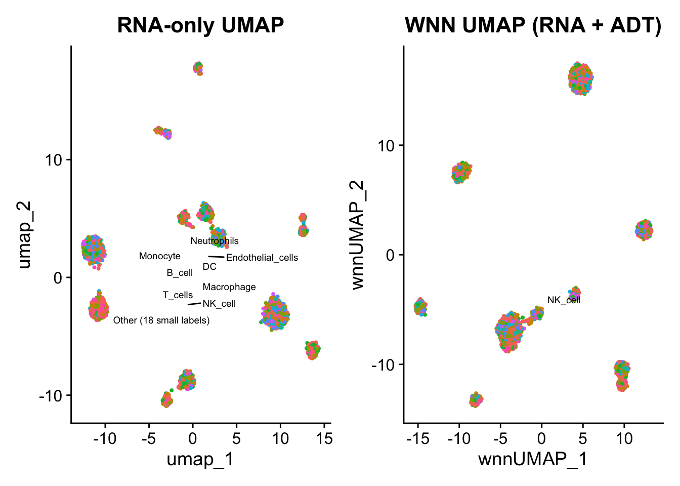
WNN does not necessarily move every cell type to a visually different region; UMAP layouts can rotate or mirror between runs even when the underlying neighborhoods barely change. The two panels below can look similar at first glance. What actually matters is whether the set of cells grouped together changed, not whether the picture looks different.

Step 6.11c (later) checks this directly per cell-type via a cross-table; here, a quick clustering comparison gives a first read before that.

Code

sobj_filt <- FindClusters(sobj_filt, resolution = 0.5,
                          cluster.name = "rna_only_clusters_preview",
                          verbose = FALSE)
rna_only_clusters <- sobj_filt$rna_only_clusters_preview

sobj_filt <- FindClusters(sobj_filt, graph.name = "wsnn", resolution = 0.5,
                          cluster.name = "wnn_clusters_preview",
                          verbose = FALSE)
wnn_clusters_preview <- sobj_filt$wnn_clusters_preview

agreement_tab <- table(RNA_only = rna_only_clusters, WNN = wnn_clusters_preview)
cat("Cluster membership: RNA-only vs WNN (rows: RNA-only clusters, cols: WNN clusters)\n")

Cluster membership: RNA-only vs WNN (rows: RNA-only clusters, cols: WNN clusters)

Code

print(agreement_tab)

        WNN
RNA_only   0   1   2   3   4   5   6   7   8
      0  527   0   0   0   0   0   0   0   0
      1    0 329   0   0 131   0   0   0   0
      2    0 254   0   0  93   0   0   0   0
      3    0   0 221   0   0   0   0   0   0
      4    0   0   0 198   0   0   0   0   0
      5    9   0   1   0   1 166   0   4  16
      6  165   0   0   0   0   0   0   0   0
      7    0   0   0   0   0   0 134   0   1
      8    0   0 118   0   0   0   0   0   0
      9    0   0   0   0   0   0   0 116   0
      10   0   0   0 107   0   0   0   0   0
      11   0   0   0   0   0   0   0   0  82

A simple agreement score: for each RNA-only cluster, what fraction of its cells land in the single WNN cluster that captures the most of them.

Code

best_match_frac <- apply(agreement_tab, 1, function(row) max(row) / sum(row))
cat(sprintf("\nMedian per-cluster agreement: %.1f%% of cells stay grouped together\n",
            100 * median(best_match_frac)))


Median per-cluster agreement: 100.0% of cells stay grouped together

Code

p_rna <- DimPlot(sobj_filt, reduction = "umap",
                 group.by = "singler_label_top",
                 label = TRUE, label.size = 2.5, repel = TRUE) +
  ggtitle("RNA-only UMAP") + NoLegend()

p_wnn <- DimPlot(sobj_filt, reduction = "wnn.umap",
                 group.by = "singler_label_top",
                 label = TRUE, label.size = 2.5, repel = TRUE) +
  ggtitle("WNN UMAP (RNA + ADT)") + NoLegend()

p_rna | p_wnn

QUESTION 6.10

If the median agreement above is high (cells mostly stay grouped the same way) but the two UMAP layouts still look visually different (different rotation, different relative positions), what does that tell you about reading UMAP plots side by side versus comparing cluster membership directly?

ANSWER

It means the visual comparison and the cluster-membership comparison are answering different questions, and only one of them is actually about whether WNN changed the result. UMAP is a 2D projection chosen independently each time it is run; rotation, mirroring, and relative spacing between blobs can differ between two UMAP runs even on the exact same underlying neighborhood graph, because UMAP’s layout optimization has no fixed orientation to anchor to. High agreement in the cluster cross-table means the cells that were grouped together under RNA-only are still grouped together under WNN, which is the substantive claim. A side-by-side UMAP comparison is useful for a first visual impression and for spotting gross differences (a population that splits or merges), but it is not a reliable way to judge subtle changes, and two UMAPs that look different are not, by themselves, evidence that WNN changed anything about which cells belong together.

LIVE DEMO:

Code

print(agreement_tab)

        WNN
RNA_only   0   1   2   3   4   5   6   7   8
      0  527   0   0   0   0   0   0   0   0
      1    0 329   0   0 131   0   0   0   0
      2    0 254   0   0  93   0   0   0   0
      3    0   0 221   0   0   0   0   0   0
      4    0   0   0 198   0   0   0   0   0
      5    9   0   1   0   1 166   0   4  16
      6  165   0   0   0   0   0   0   0   0
      7    0   0   0   0   0   0 134   0   1
      8    0   0 118   0   0   0   0   0   0
      9    0   0   0   0   0   0   0 116   0
      10   0   0   0 107   0   0   0   0   0
      11   0   0   0   0   0   0   0   0  82

Code

median(best_match_frac)   # fraction of cells staying grouped together

[1] 1

PLOT / OUTPUT: The agreement_tab cross-table and the median agreement number, alongside the two UMAP panels

5.1.14 Step 6.11 - Per-cell modality weights

RNA.weight close to 1 = cell is better characterized by RNA
RNA.weight close to 0 = cell is better characterized by ADT
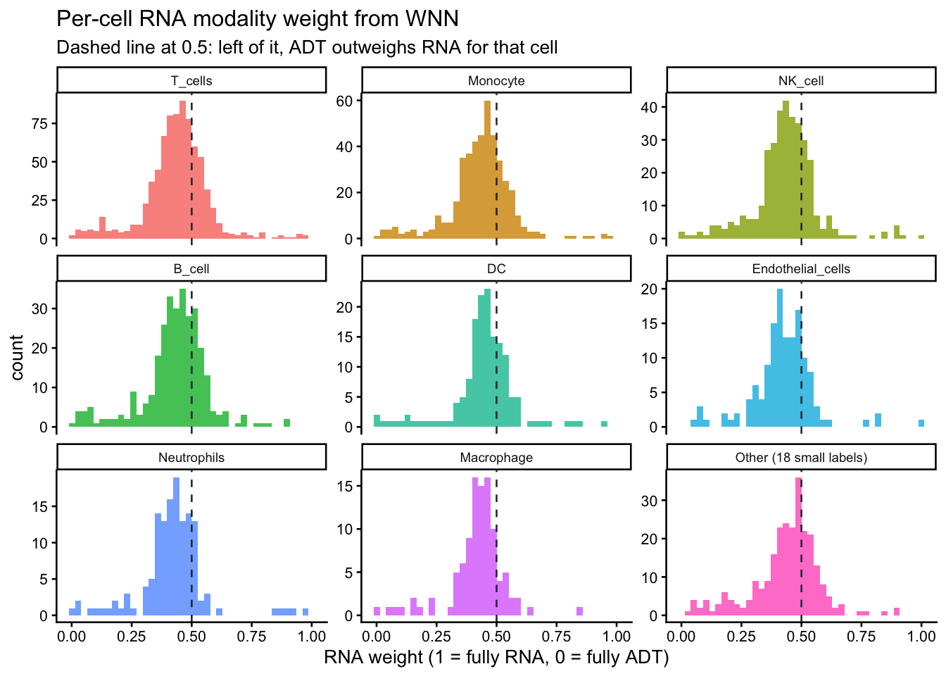
RNA.weight and ADT.weight sum to 1 for each cell (FindMultiModalNeighbors normalizes them that way), so 0.5 is the natural reference point: below it, ADT is contributing more than RNA to that cell’s placement in the WNN graph, not just “some amount” of protein information.

Code

pct_below_half <- round(mean(sobj_filt$RNA.weight < 0.5) * 100, 1)
cat(sprintf("Cells where ADT contributes more than RNA (RNA.weight < 0.5): %.1f%%\n",
            pct_below_half))

Cells where ADT contributes more than RNA (RNA.weight < 0.5): 74.8%

Code

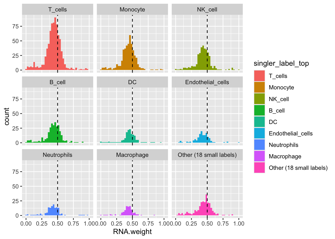
ggplot(sobj_filt@meta.data, aes(x = RNA.weight, fill = singler_label_top)) +
  geom_histogram(bins = 40, alpha = 0.8) +
  geom_vline(xintercept = 0.5, linetype = "dashed", color = "#2c3142") +
  facet_wrap(~singler_label_top, scales = "free_y") +
  labs(title    = "Per-cell RNA modality weight from WNN",
       subtitle = "Dashed line at 0.5: left of it, ADT outweighs RNA for that cell",
       x = "RNA weight (1 = fully RNA, 0 = fully ADT)") +
  theme_classic(base_size = 10) +
  theme(legend.position = "none",
        strip.text      = element_text(size = 7))

QUESTION 6.11

Which cell types in this dataset rely most on ADT (low RNA weight)? Why does that match what you know about RNA dropout for their defining markers?

ANSWER

CD4 T cells and CD8 T cells, by a wide margin. Their defining markers (CD4, CD8A) have the worst RNA dropout. B cells (MS4A1, CD79A) and monocytes (CD14, LYZ) have stronger RNA signal and rely less on ADT. NK cells (NKG7, GNLY, NCAM1) are intermediate. The histogram facet of RNA.weight by cell type makes this concrete, and the dashed line at RNA.weight = 0.5 marks the point where ADT outweighs RNA for that cell, not just contributes some amount of information.

LIVE DEMO:

Code

mean(sobj_filt$RNA.weight < 0.5) * 100   # cells where ADT outweighs RNA

[1] 74.8223

Code

ggplot(sobj_filt@meta.data, aes(x = RNA.weight, fill = singler_label_top)) +
  geom_histogram(bins = 40) + geom_vline(xintercept = 0.5, linetype = "dashed") +
  facet_wrap(~singler_label_top)

PLOT / OUTPUT: Histogram of RNA.weight faceted by cell type, with a dashed line at 0.5. T cells peak left of the line, monocytes peak right of it.

5.1.15 Step 6.11b - RNA.weight extremes per cluster: are any clusters protein-driven?

A cluster where most cells have RNA.weight near 0 is identified almost entirely by protein. That can be biology (T cell subsets, where RNA dropout is severe) or an artifact (a protein-specific batch effect concentrated in one cluster).

Code

rna_w_by_cluster <- sobj_filt@meta.data %>%
  group_by(seurat_clusters) %>%
  summarise(median_rna_w = median(RNA.weight),
            mean_rna_w   = mean(RNA.weight),
            n_cells      = n(),
            .groups = "drop") %>%
  arrange(median_rna_w)

cat("RNA.weight per cluster (sorted; low = protein-driven):\n")

RNA.weight per cluster (sorted; low = protein-driven):

Code

print(rna_w_by_cluster)

# A tibble: 9 × 4
  seurat_clusters median_rna_w mean_rna_w n_cells
  <fct>                  <dbl>      <dbl>   <int>
1 4                      0.142      0.158     225
2 1                      0.398      0.402     583
3 0                      0.435      0.445     701
4 5                      0.439      0.431     166
5 3                      0.467      0.468     305
6 6                      0.476      0.476     134
7 2                      0.484      0.490     340
8 7                      0.491      0.487     120
9 8                      0.775      0.712      99

Flag clusters where median RNA.weight < 0.3 (protein dominates)

Code

protein_driven <- rna_w_by_cluster$seurat_clusters[rna_w_by_cluster$median_rna_w < 0.3]
if (length(protein_driven) > 0) {
  cat("\nClusters where protein dominates (median RNA.weight < 0.3):\n")
  cat("  ", paste(protein_driven, collapse = ", "), "\n")
  cat("Inspect these clusters: are they T-cell subsets (expected) or",
      "something else?\n")
}


Clusters where protein dominates (median RNA.weight < 0.3):
   4 
Inspect these clusters: are they T-cell subsets (expected) or something else?

QUESTION 6.11b

For the most protein-driven cluster, what fraction of its cells were assigned to a T-cell label by SingleR? The block below computes the answer and applies the decision rule.

ANSWER

Computed in the script. Decision thresholds: >=70% T-cell -> expected RNA-dropout behavior, no action; 30-70% -> mixed, inspect ADT proteins driving the dominance; <30% -> technical artifact, check ADT batch, CLR margin, isotype background. The script applies the rule automatically and prints the verdict.

LIVE DEMO:

Code

md <- sobj_filt@meta.data
cs <- aggregate(RNA.weight ~ seurat_clusters, data = md, FUN = median)
cs[order(cs$RNA.weight), ]

  seurat_clusters RNA.weight
5               4  0.1422525
2               1  0.3982184
1               0  0.4345525
6               5  0.4393908
4               3  0.4668456
7               6  0.4761704
3               2  0.4840516
8               7  0.4906866
9               8  0.7752781

PLOT / OUTPUT: Console table.

T-cell-like SingleR labels (any case)

Code

t_cell_pattern <- "T[._ -]?cell|CD4|CD8|Tcell|T cell"

Most protein-driven cluster = smallest median RNA.weight

Code

md <- sobj_filt@meta.data
cluster_summary <- md %>%
  group_by(seurat_clusters) %>%
  summarise(median_rna_w = median(RNA.weight, na.rm = TRUE),
            n_cells      = n(),
            t_cell_frac  = mean(grepl(t_cell_pattern, singler_label,
                                      ignore.case = TRUE), na.rm = TRUE),
            .groups = "drop") %>%
  arrange(median_rna_w)

cat("\nClusters sorted by median RNA.weight (lowest = most protein-driven):\n")


Clusters sorted by median RNA.weight (lowest = most protein-driven):

Code

print(cluster_summary)

# A tibble: 9 × 4
  seurat_clusters median_rna_w n_cells t_cell_frac
  <fct>                  <dbl>   <int>       <dbl>
1 4                      0.142     225       0.276
2 1                      0.398     583       0.336
3 0                      0.435     701       0.287
4 5                      0.439     166       0.241
5 3                      0.467     305       0.272
6 6                      0.476     134       0.351
7 2                      0.484     340       0.3  
8 7                      0.491     120       0.217
9 8                      0.775      99       0.253

Code

target_cluster <- cluster_summary$seurat_clusters[1]
tfrac          <- cluster_summary$t_cell_frac[1]
mrw            <- cluster_summary$median_rna_w[1]

cat(sprintf("\nMost protein-driven cluster: %s (median RNA.weight = %.2f)\n",
            target_cluster, mrw))


Most protein-driven cluster: 4 (median RNA.weight = 0.14)

Code

cat(sprintf("Fraction of its cells with T-cell label: %.1f%%\n", tfrac * 100))

Fraction of its cells with T-cell label: 27.6%

Code

cat("\nDecision rule (concrete thresholds):\n")


Decision rule (concrete thresholds):

Code

cat("  t_cell_frac >= 70%  -> protein dominance reflects RNA dropout (expected,\n")

  t_cell_frac >= 70%  -> protein dominance reflects RNA dropout (expected,

Code

cat("                         CD4/CD8 RNA drops out heavily). No action.\n")

                         CD4/CD8 RNA drops out heavily). No action.

Code

cat("  t_cell_frac 30-70%  -> mixed. Inspect ADT panel for this cluster: is one\n")

  t_cell_frac 30-70%  -> mixed. Inspect ADT panel for this cluster: is one

Code

cat("                         specific protein driving the dominance? Run:\n")

                         specific protein driving the dominance? Run:

Code

cat("                         FeaturePlot(sobj_filt, '<protein>',\n")

                         FeaturePlot(sobj_filt, '<protein>',

Code

cat("                                     cells = WhichCells(sobj_filt, idents = '<cluster>'))\n")

                                     cells = WhichCells(sobj_filt, idents = '<cluster>'))

Code

cat("  t_cell_frac < 30%   -> technical explanation. Check:\n")

  t_cell_frac < 30%   -> technical explanation. Check:

Code

cat("                         1. ADT batch (Block 6.3, panel QC)\n")

                         1. ADT batch (Block 6.3, panel QC)

Code

cat("                         2. CLR margin (Block 6.2; verify row means != 0)\n")

                         2. CLR margin (Block 6.2; verify row means != 0)

Code

cat("                         3. Isotype background (Block 8 Scenario 4)\n")

                         3. Isotype background (Block 8 Scenario 4)

Code

verdict <- if (tfrac >= 0.70) {
  "RNA dropout (expected)"
} else if (tfrac >= 0.30) {
  "mixed; inspect ADT panel"
} else {
  "technical artifact; check batch/CLR/isotype"
}
cat(sprintf("\nVerdict for cluster %s: %s\n", target_cluster, verdict))


Verdict for cluster 4: technical artifact; check batch/CLR/isotype

5.1.16 Step 6.11c - Cell-level reannotation: WNN clustering vs RNA-only label

Run a graph-based clustering on the WNN graph and compare it to the RNA-only SingleR annotation, restricted to cells where ADT dominated.

Code

sobj_filt <- FindClusters(sobj_filt,
                          graph.name = "wsnn",
                          resolution = 0.5,
                          verbose    = FALSE)
sobj_filt$wnn_clusters <- Idents(sobj_filt)

Cells where ADT dominated WNN (RNA.weight < 0.3)

Code

low_rna_mask <- sobj_filt$RNA.weight < 0.3
n_low <- sum(low_rna_mask)
cat("Cells where ADT dominated WNN (RNA.weight < 0.3):", n_low,
    sprintf("(%.1f%% of total)\n", 100 * n_low / ncol(sobj_filt)))

Cells where ADT dominated WNN (RNA.weight < 0.3): 301 (11.3% of total)

Code

if (n_low >= 20) {
  cat("\nCross-tab: RNA-based SingleR label vs WNN cluster (ADT-dominated cells)\n")
  print(table(
    SingleR_label = sobj_filt$singler_label[low_rna_mask],
    WNN_cluster   = sobj_filt$wnn_clusters[low_rna_mask]
  ))
}


Cross-tab: RNA-based SingleR label vs WNN cluster (ADT-dominated cells)
                   WNN_cluster
SingleR_label        0  1  2  3  4  5  6  7  8
  B_cell             0 11  0  0 28  1  0  0  1
  DC                 1  4  0  0  8  1  0  0  0
  Endothelial_cells  2  4  0  0 10  0  0  0  0
  Epithelial_cells   0  2  0  0  6  0  0  0  0
  Gametocytes        0  0  0  0  1  0  0  0  0
  Hepatocytes        0  0  0  0  2  0  0  0  0
  Macrophage         1  0  0  0  8  0  0  0  1
  Monocyte           2 15  0  0 26  4  0  0  1
  Myelocyte          0  0  0  0  3  0  0  0  0
  Neurons            0  0  0  0  2  0  0  0  0
  Neutrophils        0  1  0  0 12  0  0  0  3
  NK_cell            3 13  0  0 24  1  0  0  1
  Platelets          0  1  0  0  5  0  0  0  0
  Pre-B_cell_CD34-   0  2  0  0 10  0  0  0  0
  T_cells            5 18  0  0 53  4  0  0  0

QUESTION 6.11c

For the row of the cross-table with the largest disagreement, the SingleR-RNA label and the WNN cluster diverge. Which one do you trust? The code below identifies that row automatically and runs the deciding check.

Code

if (n_low >= 20) {
  ctab <- table(
    SingleR_label = sobj_filt$singler_label[low_rna_mask],
    WNN_cluster   = sobj_filt$wnn_clusters[low_rna_mask]
  )
  # Largest off-diagonal cell = biggest disagreement
  if (length(ctab) > 1) {
    max_cell <- arrayInd(which.max(ctab), dim(ctab))
    src_lbl <- rownames(ctab)[max_cell[1]]
    src_clu <- colnames(ctab)[max_cell[2]]
    n_conf  <- ctab[max_cell[1], max_cell[2]]
    cat(sprintf("\nLargest disagreement: %d cells labeled '%s' by SingleR-RNA\n",
                n_conf, src_lbl))
    cat(sprintf("but assigned to WNN cluster %s.\n", src_clu))

    # Deciding check: marker expression in those cells.
    # T-cell markers (RNA + ADT), B-cell markers, Mono markers
    decider_markers <- list(
      T_cell    = list(rna = c("CD3E", "CD3D"), adt = c("CD3")),
      B_cell    = list(rna = c("MS4A1", "CD79A"), adt = c("CD19", "CD20")),
      Monocyte  = list(rna = c("CD14", "LYZ"),   adt = c("CD14")),
      NK_cell   = list(rna = c("NKG7", "GNLY"),  adt = c("CD56"))
    )

    conf_cells <- which(low_rna_mask &
                        sobj_filt$singler_label == src_lbl &
                        sobj_filt$wnn_clusters  == src_clu)
    cat(sprintf("Marker detection in %d disputed cells:\n", length(conf_cells)))
    for (ct in names(decider_markers)) {
      for (mk in decider_markers[[ct]]$rna) {
        if (mk %in% rownames(sobj_filt[["RNA"]])) {
          v <- FetchData(sobj_filt, vars = mk)[conf_cells, 1]
          cat(sprintf("  %s (RNA %s): %.1f%% > 0\n", ct, mk, mean(v > 0) * 100))
        }
      }
      for (mk in decider_markers[[ct]]$adt) {
        if (mk %in% rownames(sobj_filt[["ADT"]])) {
          DefaultAssay(sobj_filt) <- "ADT"
          v <- FetchData(sobj_filt, vars = mk)[conf_cells, 1]
          DefaultAssay(sobj_filt) <- "RNA"
          cat(sprintf("  %s (ADT %s): %.1f%% > 1.0 (CLR units)\n",
                      ct, mk, mean(v > 1.0) * 100))
        }
      }
    }

    cat("\nDecision rule:\n")
    cat("  The cell type whose markers fire in >= 50% of cells (RNA + ADT\n")
    cat("  combined) wins. If two cell types tie, mark these cells as\n")
    cat("  ambiguous (likely doublets that scDblFinder missed) and remove\n")
    cat("  before downstream group comparison.\n")
  }
}


Largest disagreement: 53 cells labeled 'T_cells' by SingleR-RNA
but assigned to WNN cluster 4.
Marker detection in 53 disputed cells:
  T_cell (RNA CD3E): 100.0% > 0
  T_cell (RNA CD3D): 100.0% > 0
  T_cell (ADT CD3): 100.0% > 1.0 (CLR units)
  B_cell (RNA MS4A1): 5.7% > 0
  B_cell (RNA CD79A): 1.9% > 0
  B_cell (ADT CD19): 0.0% > 1.0 (CLR units)
  B_cell (ADT CD20): 0.0% > 1.0 (CLR units)
  Monocyte (RNA CD14): 5.7% > 0
  Monocyte (RNA LYZ): 3.8% > 0
  Monocyte (ADT CD14): 0.0% > 1.0 (CLR units)
  NK_cell (RNA NKG7): 3.8% > 0
  NK_cell (RNA GNLY): 5.7% > 0
  NK_cell (ADT CD56): 0.0% > 1.0 (CLR units)

Decision rule:
  The cell type whose markers fire in >= 50% of cells (RNA + ADT
  combined) wins. If two cell types tie, mark these cells as
  ambiguous (likely doublets that scDblFinder missed) and remove
  before downstream group comparison.

ANSWER

Decision rule from the script: cross-check marker expression in the disputed cells. The cell type whose markers (RNA + ADT) fire in >=50% of cells wins. If two cell types tie, mark the cells as ambiguous (likely undetected doublets) and exclude them from downstream group comparisons. Do NOT pick the WNN label by default; do NOT pick the SingleR label by default. Let the markers adjudicate.

LIVE DEMO:

Code

low_rna_mask <- sobj_filt$RNA.weight < 0.3
tab <- table(sobj_filt$singler_label[low_rna_mask],
             sobj_filt$wnn_clusters[low_rna_mask])
tab

                   
                     0  1  2  3  4  5  6  7  8
  B_cell             0 11  0  0 28  1  0  0  1
  DC                 1  4  0  0  8  1  0  0  0
  Endothelial_cells  2  4  0  0 10  0  0  0  0
  Epithelial_cells   0  2  0  0  6  0  0  0  0
  Gametocytes        0  0  0  0  1  0  0  0  0
  Hepatocytes        0  0  0  0  2  0  0  0  0
  Macrophage         1  0  0  0  8  0  0  0  1
  Monocyte           2 15  0  0 26  4  0  0  1
  Myelocyte          0  0  0  0  3  0  0  0  0
  Neurons            0  0  0  0  2  0  0  0  0
  Neutrophils        0  1  0  0 12  0  0  0  3
  NK_cell            3 13  0  0 24  1  0  0  1
  Platelets          0  1  0  0  5  0  0  0  0
  Pre-B_cell_CD34-   0  2  0  0 10  0  0  0  0
  T_cells            5 18  0  0 53  4  0  0  0

PLOT / OUTPUT: Console cross-table.

5.1.17 Step 6.12 - Condition comparison: Healthy vs COVID-19

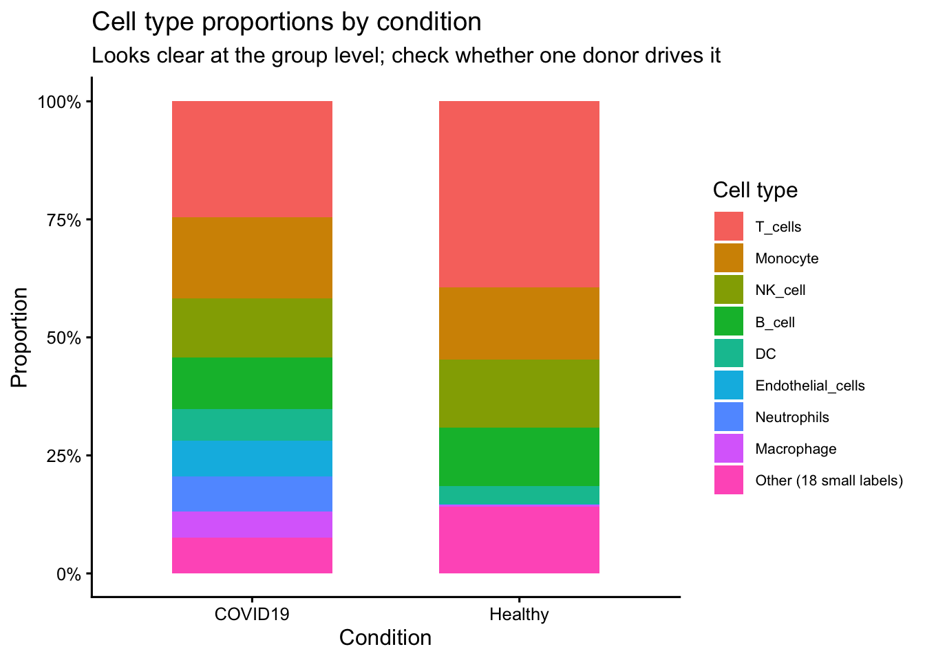
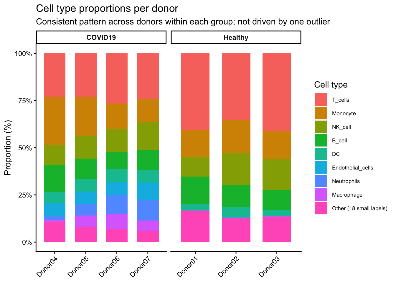
This plot looks informative. But with 3 Healthy and 4 COVID-19 donors, it can be completely driven by one outlier donor.

Code

group_props <- sobj_filt@meta.data %>%
  filter(!is.na(singler_label_top), !is.na(condition)) %>%
  group_by(condition, singler_label_top) %>%
  summarise(n = n(), .groups = "drop") %>%
  group_by(condition) %>%
  mutate(prop = n / sum(n))

ggplot(group_props, aes(x = condition, y = prop, fill = singler_label_top)) +
  geom_bar(stat = "identity", width = 0.6) +
  scale_y_continuous(labels = percent_format()) +
  labs(title    = "Cell type proportions by condition",
       subtitle = "Looks clear at the group level; check whether one donor drives it",
       x = "Condition", y = "Proportion", fill = "Cell type") +
  theme_classic(base_size = 12) +
  theme(legend.text = element_text(size = 8))

Code

donor_props <- sobj_filt@meta.data %>%
  filter(!is.na(singler_label_top)) %>%
  group_by(donor_id, condition, singler_label_top) %>%
  summarise(n = n(), .groups = "drop") %>%
  group_by(donor_id) %>%
  mutate(prop = n / sum(n))

ggplot(donor_props, aes(x = donor_id, y = prop, fill = singler_label_top)) +
  geom_bar(stat = "identity", width = 0.7) +
  scale_y_continuous(labels = percent_format()) +
  facet_wrap(~condition, scales = "free_x") +
  labs(title    = "Cell type proportions per donor",
       subtitle = "Consistent pattern across donors within each group; not driven by one outlier",
       x = NULL, y = "Proportion (%)", fill = "Cell type") +
  theme_classic(base_size = 11) +
  theme(axis.text.x = element_text(angle = 45, hjust = 1),
        legend.text = element_text(size = 7),
        strip.text  = element_text(face = "bold"))

5.1.18 Step 6.12b - Statistical reality check: donor-level test with power note

Per-donor proportions for ONE example cell type, tested between conditions. Run this for whichever label your annotation produced as the largest in COVID-19; the script tries to pick automatically.

Per-donor proportions for ONE example cell type, tested between conditions. Run this for whichever label your annotation produced as the largest in COVID-19; the script tries to pick automatically. Restricted to top-N labels: a label held by 1-2 cells could show a spurious 100% delta between conditions by chance alone, which would make a meaningless “finding” look like the strongest signal in the dataset.

Code

per_donor <- sobj_filt@meta.data %>%
  filter(!is.na(condition), !is.na(singler_label_top), condition %in% c("Healthy", "COVID19")) %>%
  group_by(donor_id, condition, singler_label_top) %>%
  summarise(n = n(), .groups = "drop") %>%
  group_by(donor_id, condition) %>%
  mutate(prop = n / sum(n)) %>%
  ungroup()

Pick the cell type with the largest delta between groups for demonstration

Code

delta_by_lbl <- per_donor %>%
  group_by(singler_label_top, condition) %>%
  summarise(mean_prop = mean(prop), .groups = "drop") %>%
  tidyr::pivot_wider(names_from = condition, values_from = mean_prop) %>%
  mutate(delta = abs(COVID19 - Healthy)) %>%
  arrange(desc(delta))

target_lbl <- delta_by_lbl$singler_label_top[1]
cat("Largest mean-proportion delta is for label:", as.character(target_lbl), "\n")

Largest mean-proportion delta is for label: T_cells

Code

cat(sprintf("  Healthy mean: %.1f%%   COVID-19 mean: %.1f%%   delta: %.1f%%\n",
            100 * delta_by_lbl$Healthy[1],
            100 * delta_by_lbl$COVID19[1],
            100 * delta_by_lbl$delta[1]))

  Healthy mean: 39.1%   COVID-19 mean: 24.4%   delta: 14.7%

Code

subset_df <- per_donor %>% filter(singler_label_top == target_lbl)
n_h <- sum(subset_df$condition == "Healthy")
n_c <- sum(subset_df$condition == "COVID19")

if (n_h >= 2 && n_c >= 2) {
  wt <- wilcox.test(prop ~ condition, data = subset_df, exact = FALSE)
  cat(sprintf("\nWilcoxon rank-sum (n=%d Healthy vs n=%d COVID-19):\n", n_h, n_c))
  cat(sprintf("  W = %g, p = %.3f\n", wt$statistic, wt$p.value))
}


Wilcoxon rank-sum (n=3 Healthy vs n=4 COVID-19):
  W = 0, p = 0.052

Power floor: with n=3 vs n=4 and Wilcoxon at alpha=0.05, the smallest detectable standardized effect size (Cohen’s d) is roughly 1.5 for 80% power.

In plain terms: only proportion differences larger than ~1.5 standard deviations of the donor-level distribution are detectable. Any p-value here is exploratory, not confirmatory.

Code

cat("\n--- Power note ---\n")


--- Power note ---

Code

cat("n=3 vs n=4 donors. Minimum detectable effect size (Cohen's d) ~1.5 for\n")

n=3 vs n=4 donors. Minimum detectable effect size (Cohen's d) ~1.5 for

Code

cat("80% power at alpha=0.05. Treat any p-value here as exploratory only.\n")

80% power at alpha=0.05. Treat any p-value here as exploratory only.

QUESTION 6.12b

Assuming the printed p-value is in the 0.05 - 0.10 range, what conclusion can you DRAW from this dataset? The block below applies the explicit decision rule for small-sample group comparison.

Code

cat("\nDecision matrix for the observed p-value:\n")


Decision matrix for the observed p-value:

Code

if (exists("wt")) {
  pv <- wt$p.value
  cat(sprintf("  Observed p-value: %.3f\n", pv))
  cat("\n  p < 0.01 with n=7 donors total: STRONG signal, replicate in a\n")
  cat("                                     larger cohort before claiming.\n")
  cat("  0.01 <= p < 0.05               : Suggestive. Report effect size +\n")
  cat("                                     per-donor plot. Not confirmatory.\n")
  cat("  0.05 <= p < 0.10               : Exploratory. Cannot claim difference.\n")
  cat("                                     State the n, the direction, and the\n")
  cat("                                     effect size; flag as hypothesis-\n")
  cat("                                     generating only.\n")
  cat("  p >= 0.10                      : No evidence of difference at this n.\n")
  cat("                                     Power analysis says n>=10 per group\n")
  cat("                                     needed for the observed effect size.\n")

  # Auto-apply
  verdict <- if (pv < 0.01) {
    "STRONG (replicate in larger cohort)"
  } else if (pv < 0.05) {
    "suggestive (report with caveats)"
  } else if (pv < 0.10) {
    "exploratory (hypothesis-generating only)"
  } else {
    "no evidence of difference at this n"
  }
  cat(sprintf("\nAutomatic verdict at p = %.3f: %s\n", pv, verdict))

  # Minimum n needed for the observed effect (Cohen's d -> n via power calc)
  pooled_sd <- sd(subset_df$prop)
  obs_d     <- delta_by_lbl$delta[1] / pooled_sd
  cat(sprintf("\nObserved Cohen's d (donor-level): %.2f\n", obs_d))
  cat("Approximate n per group needed for 80%% power at alpha=0.05:\n")
  # Rough rule: n ~= 16 / d^2 for two-sample t-test, similar for Wilcoxon
  if (!is.na(obs_d) && obs_d > 0) {
    n_needed <- ceiling(16 / obs_d^2)
    cat(sprintf("  ~%d donors per group (using rule n ~ 16/d^2)\n", n_needed))
  }
}

  Observed p-value: 0.052

  p < 0.01 with n=7 donors total: STRONG signal, replicate in a
                                     larger cohort before claiming.
  0.01 <= p < 0.05               : Suggestive. Report effect size +
                                     per-donor plot. Not confirmatory.
  0.05 <= p < 0.10               : Exploratory. Cannot claim difference.
                                     State the n, the direction, and the
                                     effect size; flag as hypothesis-
                                     generating only.
  p >= 0.10                      : No evidence of difference at this n.
                                     Power analysis says n>=10 per group
                                     needed for the observed effect size.

Automatic verdict at p = 0.052: exploratory (hypothesis-generating only)

Observed Cohen's d (donor-level): 1.80
Approximate n per group needed for 80%% power at alpha=0.05:
  ~5 donors per group (using rule n ~ 16/d^2)

Code

saveRDS(sobj_filt, "outputs/sobj_annotated.rds")
cat("Annotated object saved: outputs/sobj_annotated.rds\n")

Annotated object saved: outputs/sobj_annotated.rds

ANSWER

Exploratory only. With n=7 donors total, a p-value in this range is hypothesis-generating and cannot support a published claim of difference. Report: n per group, direction of the difference, effect size, statement that confirmatory analysis requires a larger cohort. The script estimates the n needed for 80% power at the observed effect size (rule of thumb n ~ 16 / d^2).

LIVE DEMO: See Step 6.12b (Section 5.1.18) in the script: it auto-applies the decision matrix.

PLOT / OUTPUT: Console output with automatic verdict.

QUESTION 6.12

How would you formally test the group-level difference given only 3 healthy vs 4 COVID-19 donors? What is the minimum reporting standard you would accept in a paper?

ANSWER

Donor as the unit of analysis. Compute per-donor cell-type proportions (one number per donor per cell type), Wilcoxon rank-sum across donors. With n=3 vs n=4 power is minimal: only effect sizes near Cohen’s d=1.5 are detectable at alpha=0.05. Minimum reporting standard: plot per-donor proportions (Step 6.12 does this), state the n, and explicitly mark the analysis as exploratory unless effect sizes are very large. Group-level barplots without per-donor backing should not appear in a paper.

LIVE DEMO:

Code

subset_df <- per_donor %>% filter(singler_label == target_lbl)

Error in `filter()`:
ℹ In argument: `singler_label == target_lbl`.
Caused by error:
! object 'singler_label' not found

Code

wilcox.test(prop ~ condition, data = subset_df, exact = FALSE)


    Wilcoxon rank sum test with continuity correction

data:  prop by condition
W = 0, p-value = 0.05183
alternative hypothesis: true location shift is not equal to 0

Code

print(subset_df[, c("donor_id", "condition", "prop")])

# A tibble: 7 × 3
  donor_id condition  prop
  <chr>    <chr>     <dbl>
1 Donor01  Healthy   0.407
2 Donor02  Healthy   0.354
3 Donor03  Healthy   0.413
4 Donor04  COVID19   0.233
5 Donor05  COVID19   0.233
6 Donor06  COVID19   0.266
7 Donor07  COVID19   0.244

PLOT / OUTPUT: Per-donor proportion boxplot with individual donors as points, colored by condition.

5.2 Block 7 - Closing

Final view of the annotated proportions and the R session record. The pitfalls reference table lives in the instructor’s guide PDF.

5.2.1 Step 7.1 - Four-panel summary

Four results that together summarize the course, reusing objects already built in Blocks 5 and 6 rather than recomputing anything:

Final WNN UMAP with confident annotation: the end state of the RNA + ADT integration.
Top canonical markers per cell type: the evidence behind the labels in panel 1.
Cell type proportions by condition: the biological comparison the whole pipeline was built to support.
CD4 in RNA vs ADT: the single clearest illustration from the course of why the protein layer earns its place in the analysis.

Code

p_final_umap <- DimPlot(sobj_filt, reduction = "wnn.umap",
                        group.by = "singler_label_clean",
                        label = TRUE, label.size = 2.5, repel = TRUE) +
  ggtitle("1. Final WNN UMAP (confident annotation)") + NoLegend()

p_final_markers <- DotPlot(sobj_filt,
                           features = unique(top_markers$gene),
                           idents   = setdiff(levels(Idents(sobj_filt)), "Ambiguous"),
                           group.by = "singler_label_clean") +
  RotatedAxis() +
  theme(axis.text.x = element_text(size = 7), legend.position = "none") +
  ggtitle("2. Canonical markers behind the labels")

if ("singler_label_top" %in% colnames(sobj_filt@meta.data)) {
  final_props <- sobj_filt@meta.data %>%
    filter(!is.na(condition), !is.na(singler_label_top)) %>%
    group_by(condition, singler_label_top) %>%
    summarise(n = n(), .groups = "drop") %>%
    group_by(condition) %>%
    mutate(prop = n / sum(n))

  p_final_props <- ggplot(final_props, aes(condition, prop, fill = singler_label_top)) +
    geom_bar(stat = "identity", width = 0.65) +
    scale_y_continuous(labels = percent_format()) +
    labs(x = "Condition", y = "Proportion", fill = NULL) +
    theme_classic(base_size = 10) +
    theme(legend.text = element_text(size = 6),
          legend.position = "right",
          axis.text.x = element_text(angle = 45, hjust = 1)) +
    ggtitle("3. Cell type proportions by condition")
}

DefaultAssay(sobj_filt) <- "RNA"
p_cd4_rna <- FeaturePlot(sobj_filt, "CD4", min.cutoff = "q05") +
  ggtitle("4a. CD4 (RNA)") +
  theme(plot.title = element_text(size = 10), legend.position = "none")
DefaultAssay(sobj_filt) <- "ADT"
p_cd4_adt <- FeaturePlot(sobj_filt, "CD4", min.cutoff = "q05") +
  ggtitle("4b. CD4 (ADT)") +
  theme(plot.title = element_text(size = 10), legend.position = "none")
DefaultAssay(sobj_filt) <- "RNA"
p_final_cd4 <- p_cd4_rna | p_cd4_adt

(p_final_umap | p_final_markers) / (p_final_props | p_final_cd4)

5.2.2 Step 7.2 - Session info

Code

sessionInfo()

R version 4.6.0 (2026-04-24)
Platform: aarch64-apple-darwin23
Running under: macOS Tahoe 26.5.1

Matrix products: default
BLAS:   /Library/Frameworks/R.framework/Versions/4.6/Resources/lib/libRblas.0.dylib 
LAPACK: /Library/Frameworks/R.framework/Versions/4.6/Resources/lib/libRlapack.dylib;  LAPACK version 3.12.1

locale:
[1] en_US.UTF-8/en_US.UTF-8/en_US.UTF-8/C/en_US.UTF-8/en_US.UTF-8

time zone: America/Mexico_City
tzcode source: internal

attached base packages:
[1] stats4    stats     graphics  grDevices utils     datasets  methods  
[8] base     

other attached packages:
 [1] future_1.70.0               here_1.0.2                 
 [3] ggrepel_0.9.8               scales_1.4.0               
 [5] harmony_2.0.5               Rcpp_1.1.1-1.1             
 [7] BiocParallel_1.46.0         SingleR_2.14.0             
 [9] SummarizedExperiment_1.42.0 Biobase_2.72.0             
[11] GenomicRanges_1.64.0        Seqinfo_1.2.0              
[13] IRanges_2.46.0              S4Vectors_0.50.1           
[15] BiocGenerics_0.58.1         generics_0.1.4             
[17] MatrixGenerics_1.24.0       matrixStats_1.5.0          
[19] Matrix_1.7-5                tidyr_1.3.2                
[21] dplyr_1.2.1                 patchwork_1.3.2            
[23] ggplot2_4.0.3               Seurat_5.5.1               
[25] SeuratObject_5.4.0          sp_2.2-1                   

loaded via a namespace (and not attached):
  [1] RColorBrewer_1.1-3     rstudioapi_0.19.0      jsonlite_2.0.0        
  [4] magrittr_2.0.5         ggbeeswarm_0.7.3       spatstat.utils_3.2-3  
  [7] farver_2.1.2           rmarkdown_2.31         vctrs_0.7.3           
 [10] ROCR_1.0-12            spatstat.explore_3.8-1 htmltools_0.5.9       
 [13] S4Arrays_1.12.0        SparseArray_1.12.2     sctransform_0.4.3     
 [16] parallelly_1.48.0      KernSmooth_2.23-26     htmlwidgets_1.6.4     
 [19] ica_1.0-3              plyr_1.8.9             plotly_4.12.0         
 [22] zoo_1.8-15             igraph_2.3.3           mime_0.13             
 [25] lifecycle_1.0.5        pkgconfig_2.0.3        R6_2.6.1              
 [28] fastmap_1.2.0          fitdistrplus_1.2-6     shiny_1.14.0          
 [31] digest_0.6.39          rprojroot_2.1.1        tensor_1.5.1          
 [34] RSpectra_0.16-2        irlba_2.3.7            beachmat_2.28.0       
 [37] labeling_0.4.3         progressr_0.19.0       spatstat.sparse_3.2-0 
 [40] httr_1.4.8             polyclip_1.10-7        abind_1.4-8           
 [43] compiler_4.6.0         withr_3.0.3            S7_0.2.2              
 [46] fastDummies_1.7.6      MASS_7.3-65            DelayedArray_0.38.2   
 [49] tools_4.6.0            vipor_0.4.7            lmtest_0.9-40         
 [52] otel_0.2.0             beeswarm_0.4.0         httpuv_1.6.17         
 [55] future.apply_1.20.2    goftest_1.2-3          glue_1.8.1            
 [58] nlme_3.1-169           promises_1.5.0         grid_4.6.0            
 [61] Rtsne_0.17             cluster_2.1.8.2        reshape2_1.4.5        
 [64] isoband_0.3.0          gtable_0.3.6           spatstat.data_3.1-9   
 [67] data.table_1.18.4      utf8_1.2.6             XVector_0.52.0        
 [70] spatstat.geom_3.8-1    RcppAnnoy_0.0.23       RANN_2.6.2            
 [73] pillar_1.11.1          stringr_1.6.0          limma_3.68.4          
 [76] spam_2.11-4            RcppHNSW_0.7.0         later_1.4.8           
 [79] splines_4.6.0          lattice_0.22-9         survival_3.8-6        
 [82] deldir_2.0-4           tidyselect_1.2.1       miniUI_0.1.2          
 [85] pbapply_1.7-4          knitr_1.51             gridExtra_2.3.1       
 [88] scattermore_1.2        xfun_0.59              statmod_1.5.2         
 [91] stringi_1.8.7          lazyeval_0.2.3         evaluate_1.0.5        
 [94] codetools_0.2-20       tibble_3.3.1           cli_3.6.6             
 [97] uwot_0.2.4             xtable_1.8-8           reticulate_1.46.0     
[100] globals_0.19.1         spatstat.random_3.5-0  png_0.1-9             
[103] ggrastr_1.0.2          spatstat.univar_3.2-0  parallel_4.6.0        
[106] dotCall64_1.2          listenv_1.0.0          viridisLite_0.4.3     
[109] ggridges_0.5.7         purrr_1.2.2            rlang_1.2.0           
[112] cowplot_1.2.0