6  Practical 15: Multimodal analysis and Integration

In this step, we will demonstrate the following:

• Analyzing the differences between merging vs integration of data.
• Loading and pre-processing scATAC-seq, multiome, and scRNA-seq reference datasets
• Mapping the scATAC-seq dataset using bridge integration.
• Performing joint RNA and ATAC analysis to explore the relationship between gene expression and chromatin accessibility in single-cell datasets.
• Exploring and evaluating the resulting annotations.

7 Batch Effect Correction

Variation in different Chromium Single Cell ATAC (Assay for Transposase Accessible Chromatin) samples can be affected by technical factors, such as laboratory conditions or reagent choices. These batch effects may confound true biological variation between samples. Therefore, correcting the batch effects can be useful for data analysis.

If you are combining libraries generated by Chromium Single Cell ATAC v1.1 and v2 reagents, you might observe systematic differences in chromatin structure profiles between libraries. Here, we will demonstrate how to use community-developed tools to merge and correct batch effects between Single Cell ATAC v1.1 and v2 data. The same procedure could also be used to correct other types of batch effects.

7.1 Option 1: Merging objects

When merging multiple single-cell chromatin datasets, it’s important to be aware that if peak calling was performed on each dataset independently, the peaks are unlikely to be exactly the same. We therefore need to create a common set of peaks across all the datasets to be merged.

The two datasets used in this example can be found here: dataset 1: 10k Human PBMCs, ATAC v1.1 cells and dataset 2: 10k Human PBMCs, ATAC v2 cells.

Download the datasets

From: Batch Effect Correction in Chromium Single Cell ATAC Data

Code

# Set working directory before downloading files
setwd("data")

# Download dataset 1 filtered_peak_bc_matrix.h5 file

download.file("https://cf.10xgenomics.com/samples/cell-atac/2.1.0/10k_pbmc_ATACv1p1_nextgem_Chromium_X/10k_pbmc_ATACv1p1_nextgem_Chromium_X_filtered_peak_bc_matrix.h5","10k_pbmc_ATACv1p1_nextgem_Chromium_X_filtered_peak_bc_matrix.h5")

# Download dataset 2 filtered_peak_bc_matrix.h5 file

download.file("https://cf.10xgenomics.com/samples/cell-atac/2.1.0/10k_pbmc_ATACv2_nextgem_Chromium_X/10k_pbmc_ATACv2_nextgem_Chromium_X_filtered_peak_bc_matrix.h5","10k_pbmc_ATACv2_nextgem_Chromium_X_filtered_peak_bc_matrix.h5")

7.2 Option 2: Harmony batch effect

We can use the Harmony batch effect correction algorithm (Korsunsky et al. 2019) implemented in the Signac R package. The Harmony algorithm is available on GitHub, and Signac has tutorials for integration.

Code

hm.integrated <- RunHarmony(object = unintegrated, group.by.vars = 'dataset', reduction = 'lsi', assay.use = 'peaks', project.dim = FALSE)
hm.integrated <- RunUMAP(hm.integrated, dims = 2:30, reduction = 'harmony')
DimPlot(hm.integrated, group.by = 'dataset', pt.size = 0.1)

7.3 Option 3: scATAC-seq data integration

An important first step in any integrative analysis of single-cell chromatin data is to ensure that the same features are measured in each dataset. Here, we quantify the multiome peaks in the ATAC dataset to ensure that there are common features across the two datasets. See the merge vignette for more information about merging chromatin assays.

7.4 Common peak set

If the peaks were identified independently in each experiment then they will likely not overlap perfectly. We can merge peaks from all the datasets to create a common peak set, and quantify this peak set in each experiment prior to merging the objects.

First we’ll load the peak coordinates for each experiment and convert them to genomic ranges, the use the GenomicRanges::reduce function to create a common set of peaks to quantify in each dataset.

flowchart LR    
  A(Create a common peak set) --> B(Create fragment objects)     
  A --> C(Quantify peaks in each dataset)
  C --> D(Create the objects)
  D --> E(Merge objects)
  E --> F(Merging without a \ncommon feature set)

8 scATAC-seq Downstream

flowchart LR    
  A{Integrating with scRNA-seq data} --> B(Gene activity matrix approach - \nRNA imputation)     
  A --> C(Dictionary Learning for cross-modality \nintegration - Bridge integration)
  B --> D[Check Biomarkers]
  C --> D

8.1 Option B: Dictionary Learning for cross-modality integration / Bridge integration

Broad schematic of the bridge integration workflow. From: Seurat v5, Hao et al, 2023. Nature biotechnology

8.1.1 Step 1: Load the bridge, query, and reference datasets (each modality individually)

Input files:

• 10x multiome dataset: Consisting of ~12,000 PBMC from a helthy donor. The dataset measures scRNA-seq and scATAC-seq in the same cell, and is available for download from 10x Genomics here.

• scATAC-seq Query: Represents ~10,000 PBMC from a healthy donor, and is available for download here.

• Reference from Azimuth: We load the reference (download here) from this recent paper. This reference is stored as an h5Seurat file, a format that enables on-disk storage of multimodal Seurat objects (more details on h5Seurat and SeuratDisk can be found here).

View data download code

Total 2.7 Gb

# 10x multiome dataset 
# Raw data 
wget https://cf.10xgenomics.com/samples/cell-arc/2.0.0/pbmc_granulocyte_sorted_10k/pbmc_granulocyte_sorted_10k_filtered_feature_bc_matrix.h5 
# fragments file 
wget https://cf.10xgenomics.com/samples/cell-arc/2.0.0/pbmc_granulocyte_sorted_10k/pbmc_granulocyte_sorted_10k_atac_fragments.tsv.gz 
# fragments index 
wget https://cf.10xgenomics.com/samples/cell-arc/2.0.0/pbmc_granulocyte_sorted_10k/pbmc_granulocyte_sorted_10k_atac_fragments.tsv.gz.tbi  

# scATAC-seq Query (Total 2.7 Gb) 
# Raw data  
wget https://cf.10xgenomics.com/samples/cell-atac/2.1.0/10k_pbmc_ATACv2_nextgem_Chromium_Controller/10k_pbmc_ATACv2_nextgem_Chromium_Controller_filtered_peak_bc_matrix.h5 
# metadata 
wget https://cf.10xgenomics.com/samples/cell-atac/2.1.0/10k_pbmc_ATACv2_nextgem_Chromium_Controller/10k_pbmc_ATACv2_nextgem_Chromium_Controller_singlecell.csv 
# fragments file 
wget https://cf.10xgenomics.com/samples/cell-atac/2.1.0/10k_pbmc_ATACv2_nextgem_Chromium_Controller/10k_pbmc_ATACv2_nextgem_Chromium_Controller_fragments.tsv.gz 
# fragments index 
wget https://cf.10xgenomics.com/samples/cell-atac/2.1.0/10k_pbmc_ATACv2_nextgem_Chromium_Controller/10k_pbmc_ATACv2_nextgem_Chromium_Controller_fragments.tsv.gz.tbi  

# Azimuth Reference (Total 9 Gb)
wget https://atlas.fredhutch.org/data/nygc/multimodal/pbmc_multimodal.h5seurat

Load and setup the 10x multiome object.

Code

library(Seurat)
library(Signac)
library(EnsDb.Hsapiens.v86)
library(dplyr)
library(ggplot2)
library(glmGamPoi)

# the 10x hdf5 file contains both data types.
inputdata.10x <- Read10X_h5("/brahms/hartmana/vignette_data/pbmc_cellranger_arc_2/pbmc_granulocyte_sorted_10k_filtered_feature_bc_matrix.h5")
# extract RNA and ATAC data
rna_counts <- inputdata.10x$`Gene Expression`
atac_counts <- inputdata.10x$Peaks
# Create Seurat object
obj.multi <- CreateSeuratObject(counts = rna_counts)
# Get % of mitochondrial genes
obj.multi[["percent.mt"]] <- PercentageFeatureSet(obj.multi, pattern = "^MT-")

# add the ATAC-seq assay
grange.counts <- StringToGRanges(rownames(atac_counts), sep = c(":", "-"))
grange.use <- seqnames(grange.counts) %in% standardChromosomes(grange.counts)
atac_counts <- atac_counts[as.vector(grange.use), ]
# Get gene annotations
annotations <- GetGRangesFromEnsDb(ensdb = EnsDb.Hsapiens.v86)
# Change style to UCSC
seqlevelsStyle(annotations) <- 'UCSC'
genome(annotations) <- "hg38"
# File with ATAC per fragment information file
frag.file <- "/brahms/hartmana/vignette_data/pbmc_cellranger_arc_2/pbmc_granulocyte_sorted_10k_atac_fragments.tsv.gz"
# Add in ATAC-seq data as ChromatinAssay object
chrom_assay <- CreateChromatinAssay(
  counts = atac_counts,
  sep = c(":", "-"),
  genome = 'hg38',
  fragments = frag.file,
  min.cells = 10,
  annotation = annotations
)

# Add the ATAC assay to the multiome object
obj.multi[["ATAC"]] <- chrom_assay
# Filter ATAC data based on QC metrics
obj.multi <- subset(
  x = obj.multi,
  subset = nCount_ATAC < 7e4 &
    nCount_ATAC > 5e3 &
    nCount_RNA < 25000 &
    nCount_RNA > 1000 &
    percent.mt < 20
)

We note that it is important to quantify the same set of genomic features in the query dataset as are quantified in the multi-omic bridge. We therefore requantify the set of scATAC-seq peaks using the FeatureMatrix command. This is also described in the Signac vignettes and shown below.

Load and setup the 10x scATAC-seq query.

Code

# Load ATAC dataset
atac_pbmc_data <- Read10X_h5(filename = "data/10k_PBMC_ATAC_nextgem_Chromium_X_filtered_peak_bc_matrix.h5") 
fragpath <- "data/10k_PBMC_ATAC_nextgem_Chromium_X_fragments.tsv.gz"
# Get gene annotations
annotation <- GetGRangesFromEnsDb(ensdb = EnsDb.Hsapiens.v86)
# Change to UCSC style 
seqlevelsStyle(annotation) <- 'UCSC'
# Create ChromatinAssay for ATAC data
atac_pbmc_assay <- CreateChromatinAssay(
  counts = atac_pbmc_data,
  sep = c(":", "-"),
  fragments = fragpath,
  annotation = annotation
)
# Requantify query ATAC to have same features as multiome ATAC dataset
requant_multiome_ATAC <- FeatureMatrix(
  fragments = Fragments(atac_pbmc_assay),
  features = granges(obj.multi[['ATAC']]),
  cells = Cells(atac_pbmc_assay)
)
# Create assay with requantified ATAC data
ATAC_assay <- CreateChromatinAssay(
  counts = requant_multiome_ATAC,
  fragments = fragpath,
  annotation = annotation
)
# Create Seurat sbject
obj.atac  <- CreateSeuratObject(counts = ATAC_assay,assay = 'ATAC')
obj.atac[['peak.orig']] <- atac_pbmc_assay
obj.atac <- subset(obj.atac, subset = nCount_ATAC < 7e4 & nCount_ATAC > 2000)

Download Azimuth reference and load it.

Code

obj.rna <- readRDS("data/pbmc_multimodal_2023.rds")

8.1.2 Step 2: Preprocessing/normalization for all datasets

Prior to performing bridge integration, we normalize and pre-process each of the datasets (note that the reference has already been normalized). We normalize gene expression data using sctransform, and ATAC data using TF-IDF.

Code

# normalize multiome RNA
DefaultAssay(obj.multi) <- "RNA"
obj.multi <- SCTransform(obj.multi, verbose = FALSE)
# normalize multiome ATAC
DefaultAssay(obj.multi) <- "ATAC"
obj.multi <- RunTFIDF(obj.multi)
obj.multi <- FindTopFeatures(obj.multi, min.cutoff = "q0")
# normalize query
obj.atac <- RunTFIDF(obj.atac)

8.1.3 Step 3: Map scATAC-seq dataset using bridge integration

Now that we have the reference, query, and bridge datasets set up, we can begin integration. The bridge dataset enables translation between the scRNA-seq reference and the scATAC-seq query, effectively augmenting the reference so that it can map a new data type. We call this an extended reference, and first set it up. Note that you can save the results of this function and map multiple scATAC-seq datasets without having to rerun.

First, we drop the first dimension of the ATAC reduction.

Code

dims.atac <- 2:50
dims.rna <- 1:50
DefaultAssay(obj.multi) <-  "RNA"
DefaultAssay(obj.rna) <- "SCT"
obj.rna.ext <- PrepareBridgeReference(
  reference = obj.rna, bridge = obj.multi,
  reference.reduction = "spca", reference.dims = dims.rna,
  normalization.method = "SCT")

Now, we can directly find anchors between the extended reference and query objects. We use the FindBridgeTransferAnchors function, which translates the query dataset using the same dictionary as was used to translate the reference, and then identifies anchors in this space. The function is meant to mimic our FindTransferAnchors function, but to identify correspondences across modalities.

Code

bridge.anchor <- FindBridgeTransferAnchors(
  extended.reference = obj.rna.ext, query = obj.atac,
  reduction = "lsiproject", dims = dims.atac)

Once we have identified anchors, we can map the query dataset onto the reference. The MapQuery function is the same as we have previously introduced for reference mapping . It transfers cell annotations from the reference dataset, and also visualizes the query dataset on a previously computed UMAP embedding. Since our reference dataset contains cell type annotations at three levels of resolution (l1 - l3), we can transfer each level to the query dataset.

Code

obj.atac <- MapQuery(
  anchorset = bridge.anchor, reference = obj.rna.ext,
  query = obj.atac,
  refdata = list(
    l1 = "celltype.l1",
    l2 = "celltype.l2",
    l3 = "celltype.l3"),
  reduction.model = "wnn.umap")

Now we can visualize the results, plotting the scATAC-seq cells based on their predicted annotations, on the reference UMAP embedding. You can see that each scATAC-seq cell has been assigned a cell name based on the scRNA-seq defined cell ontology.

Code

# plot
DimPlot(
  obj.atac, group.by = "predicted.l2",
  reduction = "ref.umap", label = TRUE
) + ggtitle("ATAC") + NoLegend()

8.1.4 Step 4: Assessing the mapping

To assess the mapping and cell type predictions, we will first see if the predicted cell type labels are concordant with an unsupervised analysis of the scATAC-seq dataset. We follow the standard unsupervised processing workflow for scATAC-seq data:

Code

obj.atac <- FindTopFeatures(obj.atac, min.cutoff = "q0")
obj.atac <- RunSVD(obj.atac)
obj.atac <- RunUMAP(obj.atac, reduction = "lsi", dims = 2:50)

Now, we visualize the predicted cluster labels on the unsupervised UMAP emebdding. We can see that predicted cluster labels (from the scRNA-seq reference) are concordant with the structure of the scATAC-seq data. However, there are some cell types (i.e. Treg), that do not appear to separate in unsupervised analysis. These may be prediction errors, or cases where the reference mapping provides additional resolution.

Code

DimPlot(obj.atac, group.by = "predicted.l2", reduction = "umap", label = FALSE)

Lastly, we validate the predicted cell types for the scATAC-seq data by examining their chromatin accessibility profiles at canonical loci. We use the CoveragePlot function to visualize accessibility patterns at the CD8A, FOXP3, and RORC, after grouping cells by their predicted labels. We see expected patterns in each case. For example, the PAX5 locus exhibits peaks that are accessible exclusively in B cells, and the CD8A locus shows the same in CD8 T cell subsets. Similarly, the accessibility of FOXP3, a canonical marker of regulatory T cells (Tregs), in predicted Tregs provides strong support for the accuracy of our prediction.

Code

CoveragePlot(
  obj.atac, region  = "PAX5", group.by = "predicted.l1",
  idents = c("B", "CD4 T", "Mono", "NK"), window = 200,
  extend.upstream = -150000)

9 Analysis of multi-omics data

Recently, single cell multi-omics methods that run several assays on the same cells have become available. One such method is Chromium Single Cell Multiome from 10X genomics, which simultaneously measures gene expression (RNA-seq) and chromatin accessibility (ATAC-seq) in the same nuclei. This makes it possible to identify cell types and states based on both gene expression and accessibility. It also makes it easy to use external gene expression data to annotate your cells, and at the same time study the chromatin accessibility in the cells.

9.1 Joint RNA and ATAC analysis: 10x multiomic

In this tutorial, we’ll demonstrate how to jointly analyze a single-cell dataset measuring both DNA accessibility and gene expression in the same cells using Signac and Seurat. In this vignette we’ll be using a publicly available 10x Genomic Multiome dataset for human PBMCs.

9.2 Dataset overview

Libraries generated:

• Chromium Single Cell Multiome ATAC library

• Chromium Single Cell Multiome Gene Expression library

View data download code

# multiomic data  
wget https://cf.10xgenomics.com/samples/cell-arc/1.0.0/pbmc_granulocyte_sorted_10k/pbmc_granulocyte_sorted_10k_filtered_feature_bc_matrix.h5
# fragments file 
wget https://cf.10xgenomics.com/samples/cell-arc/1.0.0/pbmc_granulocyte_sorted_10k/pbmc_granulocyte_sorted_10k_atac_fragments.tsv.gz
# fragments index 
wget https://cf.10xgenomics.com/samples/cell-arc/1.0.0/pbmc_granulocyte_sorted_10k/pbmc_granulocyte_sorted_10k_atac_fragments.tsv.gz.tbi

9.2.1 📗 Step 1: Load the data and create the Seurat object

Code

library(Signac)
library(Seurat)
library(EnsDb.Hsapiens.v86) # Ensembl based annotation package (hg37)
# BiocManager::install("BSgenome.Hsapiens.UCSC.hg38")
library(BSgenome.Hsapiens.UCSC.hg38) # Full genomic sequences for Homo sapiens (UCSC genome hg38)

Code

library(future)

Attaching package: 'future'

The following object is masked from 'package:AnnotationFilter':

    value

Code

# parallelization options
plan("multicore", workers = 8)
# Increase the maximum memory usage
options(future.globals.maxSize = 14 * 1024^3)  # para 14 GB de RAM

Load data and add annotation:

Code

# load the RNA and ATAC data
counts <- Read10X_h5("data/pbmc_granulocyte_sorted_10k_filtered_feature_bc_matrix.h5")
fragpath <- "data/pbmc_granulocyte_sorted_10k_atac_fragments.tsv.gz"
# get gene annotations for hg38
annotation <- GetGRangesFromEnsDb(ensdb = EnsDb.Hsapiens.v86)
seqlevels(annotation) <- paste0('chr', seqlevels(annotation))

# create a Seurat object containing the RNA adata
pbmc <- CreateSeuratObject(
  counts = counts$`Gene Expression`,
  assay = "RNA"
)

# create ATAC assay and add it to the object
pbmc[["ATAC"]] <- CreateChromatinAssay(
  counts = counts$Peaks,
  sep = c(":", "-"),
  fragments = fragpath,
  annotation = annotation
)

View file:

Code

pbmc

An object of class Seurat 
180488 features across 11898 samples within 2 assays 
Active assay: RNA (36601 features, 0 variable features)
 1 layer present: counts
 1 other assay present: ATAC

9.2.2 📕 Step 2: Computing QC metrics

We can compute per-cell quality control metrics using the DNA accessibility data and remove cells that are outliers for these metrics, as well as cells with low or unusually high counts for either the RNA or ATAC assay.

Code

DefaultAssay(pbmc) <- "ATAC"

pbmc <- NucleosomeSignal(pbmc)
pbmc <- TSSEnrichment(pbmc)

Extracting TSS positions

Extracting fragments at TSSs

Computing TSS enrichment score

The relationship between variables stored in the object metadata can be visualized using the DensityScatter() function. This can also be used to quickly find suitable cutoff values for different QC metrics by setting quantiles=TRUE:

Code

DensityScatter(pbmc, x = 'nCount_ATAC', y = 'TSS.enrichment', log_x = TRUE, quantiles = TRUE)

We can plot the distribution of each QC metric separately using a violin plot:

Code

VlnPlot(
  object = pbmc,
  features = c("nCount_RNA", "nCount_ATAC", "TSS.enrichment", "nucleosome_signal"),
  ncol = 4,
  pt.size = 0
)

Finally we remove cells that are outliers for these QC metrics. The exact QC thresholds used will need to be adjusted according to your dataset.

Code

# filter out low quality cells
pbmc <- subset(
  x = pbmc,
  subset = nCount_ATAC < 100000 &
    nCount_RNA < 25000 &
    nCount_ATAC > 1800 &
    nCount_RNA > 1000 &
    nucleosome_signal < 2 &
    TSS.enrichment > 1
)
pbmc

An object of class Seurat 
180488 features across 11211 samples within 2 assays 
Active assay: ATAC (143887 features, 0 variable features)
 2 layers present: counts, data
 1 other assay present: RNA

9.2.3 📘 Step 3: Analysis on the RNA assay

We can normalize the gene expression data using SCTransform, and reduce the dimensionality using PCA.

Code

DefaultAssay(pbmc) <- "RNA"
pbmc <- SCTransform(pbmc)

Running SCTransform on assay: RNA

Running SCTransform on layer: counts

vst.flavor='v2' set. Using model with fixed slope and excluding poisson genes.

Variance stabilizing transformation of count matrix of size 24459 by 11211

Model formula is y ~ log_umi

Get Negative Binomial regression parameters per gene

Using 2000 genes, 5000 cells

Found 167 outliers - those will be ignored in fitting/regularization step

Second step: Get residuals using fitted parameters for 24459 genes

Computing corrected count matrix for 24459 genes

Calculating gene attributes

Wall clock passed: Time difference of 1.82833 mins

Determine variable features

Centering data matrix

Getting residuals for block 1(of 3) for counts dataset

Getting residuals for block 2(of 3) for counts dataset

Getting residuals for block 3(of 3) for counts dataset

Centering data matrix

Finished calculating residuals for counts

Set default assay to SCT

Code

pbmc <- RunPCA(pbmc)

PC_ 1 
Positive:  VCAN, SAT1, PLXDC2, SLC8A1, NEAT1, DPYD, ZEB2, NAMPT, LRMDA, LYZ 
       FCN1, AOAH, LYN, ANXA1, CD36, JAK2, ARHGAP26, TYMP, RBM47, PID1 
       PLCB1, LRRK2, ACSL1, LYST, IRAK3, DMXL2, MCTP1, TCF7L2, AC020916.1, GAB2 
Negative:  EEF1A1, RPL13, RPS27, RPL13A, RPL41, RPS27A, RPS2, RPL3, RPS12, RPL11 
       RPS18, BCL2, LEF1, BCL11B, RPL23A, RPL10, BACH2, IL32, RPL34, INPP4B 
       RPS3, CAMK4, IL7R, RPS26, RPS14, RPL30, RPL19, LTB, RPLP2, SKAP1 
PC_ 2 
Positive:  GNLY, CCL5, NKG7, CD247, IL32, PRKCH, PRF1, BCL11B, INPP4B, LEF1 
       VCAN, IL7R, DPYD, THEMIS, GZMA, NEAT1, CAMK4, RORA, AOAH, PLCB1 
       TXK, GZMH, TC2N, TRBC1, ANXA1, FYB1, STAT4, PITPNC1, TRAC, AAK1 
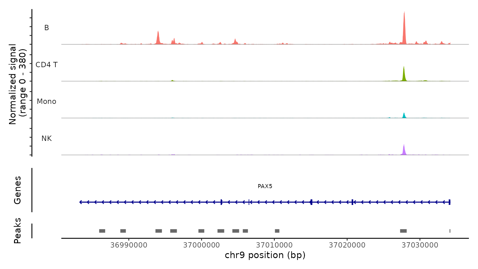
Negative:  BANK1, IGHM, AFF3, IGKC, RALGPS2, MS4A1, CD74, PAX5, EBF1, FCRL1 
       CD79A, OSBPL10, LINC00926, COL19A1, BLK, NIBAN3, IGHD, CD22, HLA-DRA, CD79B 
       ADAM28, PLEKHG1, AP002075.1, COBLL1, LIX1-AS1, CCSER1, TCF4, BCL11A, STEAP1B, GNG7 
PC_ 3 
Positive:  LEF1, CAMK4, EEF1A1, MAML2, PDE3B, FHIT, BACH2, IL7R, INPP4B, TSHZ2 
       SERINC5, NELL2, CCR7, BCL2, ANK3, PRKCA, FOXP1, TCF7, BCL11B, AC139720.1 
       RPL11, LTB, RPL13, OXNAD1, RPS27A, MLLT3, TRABD2A, RPS12, RASGRF2, VCAN 
Negative:  GNLY, NKG7, CCL5, PRF1, GZMA, GZMH, KLRD1, SPON2, FGFBP2, CST7 
       GZMB, CCL4, TGFBR3, KLRF1, CTSW, BNC2, PDGFD, ADGRG1, PPP2R2B, PYHIN1 
       A2M, IL2RB, CLIC3, MCTP2, NCAM1, ACTB, TRDC, SAMD3, NCALD, MYBL1 
PC_ 4 
Positive:  BANK1, IGHM, VCAN, IGKC, PAX5, MS4A1, GNLY, FCRL1, RALGPS2, EBF1 
       LINC00926, CD79A, OSBPL10, COL19A1, NKG7, ARHGAP24, CCL5, IGHD, BACH2, PLCB1 
       PDE4D, DPYD, LIX1-AS1, CD22, LARGE1, PLEKHG1, PLXDC2, STEAP1B, ANXA1, AP002075.1 
Negative:  TCF4, LINC01374, CUX2, AC023590.1, RHEX, PLD4, EPHB1, LINC01478, PTPRS, LINC00996 
       ZFAT, LILRA4, CLEC4C, COL26A1, FAM160A1, CCDC50, PLXNA4, ITM2C, SCN9A, COL24A1 
       UGCG, RUNX2, NRP1, GZMB, IRF8, SLC35F3, JCHAIN, BCL11A, TNFRSF21, AC007381.1 
PC_ 5 
Positive:  CDKN1C, FCGR3A, TCF7L2, IFITM3, MTSS1, AIF1, CST3, LST1, MS4A7, WARS 
       PSAP, ACTB, SERPINA1, HLA-DPA1, IFI30, CD74, COTL1, FCER1G, CFD, HLA-DRA 
       FTL, HLA-DRB1, SMIM25, CSF1R, TMSB4X, FMNL2, SAT1, MAFB, S100A4, HLA-DPB1 
Negative:  VCAN, TCF4, PLCB1, LINC01374, RHEX, CUX2, AC023590.1, DPYD, EPHB1, LINC01478 
       PTPRS, ANXA1, ZFAT, LINC00996, CD36, GZMB, PLXDC2, ARHGAP26, FCHSD2, COL26A1 
       CLEC4C, LILRA4, ACSL1, PLXNA4, AC020916.1, DYSF, ARHGAP24, CSF3R, LRMDA, MEGF9 

Caution

If you have this error:

“Error in getGlobalsAndPackages(expr, envir = envir, globals = globals) :

The total size of the 19 globals exported for future expression (‘FUN()’) is 4.69 GiB.. This exceeds the maximum allowed size of 500.00 MiB (option ‘future.globals.maxSize’). The three largest globals are ‘FUN’ (4.67 GiB of class ‘function’), ‘umi_bin’ (19.28 MiB of class ‘numeric’) and ‘data_step1’ (1.27 MiB of class ‘list’)“

You need to use parallelization in Seurat with future. If you want know more about this read this issue and documentation.

9.2.4 📙 Step 4: Analysis on the ATAC assay

Here we process the DNA accessibility assay the same way we would process a scATAC-seq dataset, by performing latent semantic indexing (LSI).

Code

# Normalization and linear dimensional reduction (LSI)
DefaultAssay(pbmc) <- "ATAC"
pbmc <- FindTopFeatures(pbmc, min.cutoff = 5)
pbmc <- RunTFIDF(pbmc)

Performing TF-IDF normalization

Code

pbmc <- RunSVD(pbmc)

Running SVD

Scaling cell embeddings

9.2.5 ✒️ Step 5: Annotating cell types

To annotate cell types in the dataset we can transfer cell labels from an existing PBMC reference dataset using tools in the Seurat package. See the Seurat reference mapping vignette for more information.

We’ll use an annotated PBMC reference dataset from Hao et al. (2020), available for download here: https://atlas.fredhutch.org/data/nygc/multimodal/pbmc_multimodal.h5seurat

Note that the SeuratDisk package is required to load the reference dataset. Installation instructions for SeuratDisk can be found here.

Install Seurat-disk

SeuratDisk is not currently available on CRAN. You can install it from GitHub with:

Code

if (!requireNamespace("remotes", quietly = TRUE)) {
  install.packages("remotes")
}
remotes::install_github("mojaveazure/seurat-disk")

If you have problems you can use this way, from this issue:

• Download the package source locally (bash terminal):

cd ~/
git clone https://github.com/mojaveazure/seurat-disk

• Install package from source:

Code

install.packages("~/seurat-disk", repos = NULL, type = "source")

Code

library(SeuratDisk)

Registered S3 method overwritten by 'SeuratDisk':
  method            from  
  as.sparse.H5Group Seurat

Code

# load PBMC reference
reference <- LoadH5Seurat("data/pbmc_multimodal.h5seurat", assays = list("SCT" = "counts"), reductions = 'spca')

Validating h5Seurat file

Initializing SCT with counts

Adding variable feature information for SCT

Adding miscellaneous information for SCT

Adding reduction spca

Adding cell embeddings for spca

Adding feature loadings for spca

Adding miscellaneous information for spca

Adding graph wknn

Adding graph wsnn

Adding command information

Adding cell-level metadata

Code

reference <- UpdateSeuratObject(reference)

Validating object structure

Updating object slots

Ensuring keys are in the proper structure

Updating matrix keys for DimReduc 'spca'

Ensuring keys are in the proper structure

Ensuring feature names don't have underscores or pipes

Updating slots in SCT

Updating slots in wknn

Cannot find wknn in the object, setting default assay of wknn to SCT

Updating slots in wsnn

Cannot find wsnn in the object, setting default assay of wsnn to SCT

Updating slots in spca

Validating object structure for SCTAssay 'SCT'

Validating object structure for Graph 'wknn'

Validating object structure for Graph 'wsnn'

Validating object structure for DimReduc 'spca'

Object representation is consistent with the most current Seurat version

Code

DefaultAssay(pbmc) <- "SCT"

# transfer cell type labels from reference to query
transfer_anchors <- FindTransferAnchors(
  reference = reference,
  query = pbmc,
  normalization.method = "SCT",
  reference.reduction = "spca",
  recompute.residuals = FALSE,
  dims = 1:50
)

Projecting cell embeddings

Finding neighborhoods

Finding anchors

    Found 14597 anchors

Code

predictions <- TransferData(
  anchorset = transfer_anchors, 
  refdata = reference$celltype.l2,
  weight.reduction = pbmc[['pca']],
  dims = 1:50
)

Finding integration vectors

Finding integration vector weights

Predicting cell labels

Code

pbmc <- AddMetaData(
  object = pbmc,
  metadata = predictions
)

# set the cell identities to the cell type predictions
Idents(pbmc) <- "predicted.id"

# remove low-quality predictions
pbmc <- pbmc[, pbmc$prediction.score.max > 0.5]

9.2.6 📐 Step 6: Joint UMAP visualization

Using the weighted nearest neighbor methods in Seurat v4, we can compute a joint neighbor graph that represent both the gene expression and DNA accessibility measurements.

Code

# build a joint neighbor graph using both assays
pbmc <- FindMultiModalNeighbors(
  object = pbmc,
  reduction.list = list("pca", "lsi"), 
  dims.list = list(1:50, 2:40),
  modality.weight.name = "RNA.weight",
  verbose = TRUE
)

Calculating cell-specific modality weights

Finding 20 nearest neighbors for each modality.

Calculating kernel bandwidths

Warning in FindMultiModalNeighbors(object = pbmc, reduction.list = list("pca",
: The number of provided modality.weight.name is not equal to the number of
modalities. SCT.weight ATAC.weight are used to store the modality weights

Finding multimodal neighbors

Constructing multimodal KNN graph

Constructing multimodal SNN graph

Code

# build a joint UMAP visualization
pbmc <- RunUMAP(
  object = pbmc,
  nn.name = "weighted.nn",
  assay = "RNA",
  verbose = TRUE
)

Warning: The default method for RunUMAP has changed from calling Python UMAP via reticulate to the R-native UWOT using the cosine metric
To use Python UMAP via reticulate, set umap.method to 'umap-learn' and metric to 'correlation'
This message will be shown once per session

18:31:32 UMAP embedding parameters a = 0.9922 b = 1.112

18:31:38 Commencing smooth kNN distance calibration using 8 threads with target n_neighbors = 20
18:31:41 Found 2 connected components, falling back to random initialization
18:31:41 Initializing from uniform random
18:31:41 Commencing optimization for 200 epochs, with 316712 positive edges
18:31:55 Optimization finished

Code

DimPlot(pbmc, label = TRUE, repel = TRUE, reduction = "umap") + NoLegend()

9.2.7 📊 Step 7: Linking peaks to genes

For each gene, we can find the set of peaks that may regulate the gene by by computing the correlation between gene expression and accessibility at nearby peaks, and correcting for bias due to GC content, overall accessibility, and peak size. See the Signac paper for a full description of the method we use to link peaks to genes.

Running this step on the whole genome can be time consuming, so here we demonstrate peak-gene links for a subset of genes as an example. The same function can be used to find links for all genes by omitting the genes.use parameter:

Code

DefaultAssay(pbmc) <- "ATAC"

# first compute the GC content for each peak
pbmc <- RegionStats(pbmc, genome = BSgenome.Hsapiens.UCSC.hg38)

Warning in RegionStats.default(object = regions, genome = genome, verbose =
verbose, : Not all seqlevels present in supplied genome

Code

# link peaks to genes
pbmc <- LinkPeaks(
  object = pbmc,
  peak.assay = "ATAC",
  expression.assay = "SCT",
  genes.use = c("LYZ", "MS4A1")
)

Testing 2 genes and 143871 peaks

Warning in .merge_two_Seqinfo_objects(x, y): Each of the 2 combined objects has sequence levels not in the other:
  - in 'x': GL000194.1, GL000195.1, GL000205.2, GL000219.1, KI270711.1, KI270713.1, KI270721.1, KI270726.1, KI270727.1, KI270728.1, KI270731.1, KI270734.1
  - in 'y': chrMT
  Make sure to always combine/compare objects based on the same reference
  genome (use suppressWarnings() to suppress this warning).

Warning: UNRELIABLE VALUE: One of the 'future.apply' iterations
('future_lapply-1') unexpectedly generated random numbers without declaring so.
There is a risk that those random numbers are not statistically sound and the
overall results might be invalid. To fix this, specify 'future.seed=TRUE'. This
ensures that proper, parallel-safe random numbers are produced via the
L'Ecuyer-CMRG method. To disable this check, use 'future.seed = NULL', or set
option 'future.rng.onMisuse' to "ignore".

Warning: UNRELIABLE VALUE: One of the 'future.apply' iterations
('future_lapply-2') unexpectedly generated random numbers without declaring so.
There is a risk that those random numbers are not statistically sound and the
overall results might be invalid. To fix this, specify 'future.seed=TRUE'. This
ensures that proper, parallel-safe random numbers are produced via the
L'Ecuyer-CMRG method. To disable this check, use 'future.seed = NULL', or set
option 'future.rng.onMisuse' to "ignore".

We can visualize these links using the CoveragePlot() function, or alternatively we could use the CoverageBrowser() function in an interactive analysis:

Code

idents.plot <- c("B naive", "B intermediate", "B memory",
                 "CD14 Mono", "CD16 Mono", "CD8 TEM", "CD8 Naive")

pbmc <- SortIdents(pbmc)

Creating pseudobulk profiles for 27 variables across 143887 features

Computing euclidean distance between pseudobulk profiles

Clustering distance matrix

Code

p1 <- CoveragePlot(
  object = pbmc,
  region = "MS4A1",
  features = "MS4A1",
  expression.assay = "SCT",
  idents = idents.plot,
  extend.upstream = 500,
  extend.downstream = 10000
)

p2 <- CoveragePlot(
  object = pbmc,
  region = "LYZ",
  features = "LYZ",
  expression.assay = "SCT",
  idents = idents.plot,
  extend.upstream = 8000,
  extend.downstream = 5000
)

patchwork::wrap_plots(p1, p2, ncol = 1)

Code

sessionInfo()

R version 4.4.1 (2024-06-14 ucrt)
Platform: x86_64-w64-mingw32/x64
Running under: Windows 11 x64 (build 22631)

Matrix products: default


locale:
[1] LC_COLLATE=English_United States.utf8 
[2] LC_CTYPE=English_United States.utf8   
[3] LC_MONETARY=English_United States.utf8
[4] LC_NUMERIC=C                          
[5] LC_TIME=English_United States.utf8    

time zone: America/Mexico_City
tzcode source: internal

attached base packages:
[1] stats4    stats     graphics  grDevices utils     datasets  methods  
[8] base     

other attached packages:
 [1] SeuratDisk_0.0.0.9021             future_1.34.0                    
 [3] BSgenome.Hsapiens.UCSC.hg38_1.4.5 BSgenome_1.72.0                  
 [5] rtracklayer_1.64.0                BiocIO_1.14.0                    
 [7] Biostrings_2.72.1                 XVector_0.44.0                   
 [9] EnsDb.Hsapiens.v86_2.99.0         ensembldb_2.28.1                 
[11] AnnotationFilter_1.28.0           GenomicFeatures_1.56.0           
[13] AnnotationDbi_1.66.0              Biobase_2.64.0                   
[15] GenomicRanges_1.56.1              GenomeInfoDb_1.40.1              
[17] IRanges_2.38.1                    S4Vectors_0.42.1                 
[19] BiocGenerics_0.50.0               Seurat_5.1.0                     
[21] SeuratObject_5.0.2                sp_2.1-4                         
[23] Signac_1.14.0                    

loaded via a namespace (and not attached):
  [1] RcppAnnoy_0.0.22            splines_4.4.1              
  [3] later_1.3.2                 bitops_1.0-8               
  [5] tibble_3.2.1                polyclip_1.10-7            
  [7] rpart_4.1.23                XML_3.99-0.17              
  [9] fastDummies_1.7.4           lifecycle_1.0.4            
 [11] hdf5r_1.3.11                globals_0.16.3             
 [13] lattice_0.22-6              MASS_7.3-60.2              
 [15] backports_1.5.0             magrittr_2.0.3             
 [17] Hmisc_5.1-3                 plotly_4.10.4              
 [19] rmarkdown_2.28              yaml_2.3.10                
 [21] httpuv_1.6.15               glmGamPoi_1.16.0           
 [23] sctransform_0.4.1           spam_2.10-0                
 [25] spatstat.sparse_3.1-0       reticulate_1.39.0          
 [27] cowplot_1.1.3               pbapply_1.7-2              
 [29] DBI_1.2.3                   RColorBrewer_1.1-3         
 [31] abind_1.4-8                 zlibbioc_1.50.0            
 [33] Rtsne_0.17                  purrr_1.0.2                
 [35] biovizBase_1.52.0           RCurl_1.98-1.16            
 [37] nnet_7.3-19                 tweenr_2.0.3               
 [39] VariantAnnotation_1.50.0    GenomeInfoDbData_1.2.12    
 [41] ggrepel_0.9.6               irlba_2.3.5.1              
 [43] listenv_0.9.1               spatstat.utils_3.1-0       
 [45] goftest_1.2-3               RSpectra_0.16-2            
 [47] spatstat.random_3.3-2       fitdistrplus_1.2-1         
 [49] parallelly_1.38.0           DelayedMatrixStats_1.26.0  
 [51] leiden_0.4.3.1              codetools_0.2-20           
 [53] DelayedArray_0.30.1         RcppRoll_0.3.1             
 [55] ggforce_0.4.2               tidyselect_1.2.1           
 [57] UCSC.utils_1.0.0            farver_2.1.2               
 [59] base64enc_0.1-3             matrixStats_1.4.0          
 [61] spatstat.explore_3.3-2      GenomicAlignments_1.40.0   
 [63] jsonlite_1.8.8              Formula_1.2-5              
 [65] progressr_0.14.0            ggridges_0.5.6             
 [67] survival_3.6-4              tools_4.4.1                
 [69] ica_1.0-3                   Rcpp_1.0.13                
 [71] glue_1.7.0                  gridExtra_2.3              
 [73] SparseArray_1.4.8           xfun_0.48                  
 [75] MatrixGenerics_1.16.0       dplyr_1.1.4                
 [77] withr_3.0.1                 fastmap_1.2.0              
 [79] fansi_1.0.6                 digest_0.6.36              
 [81] R6_2.5.1                    mime_0.12                  
 [83] colorspace_2.1-1            scattermore_1.2            
 [85] tensor_1.5                  dichromat_2.0-0.1          
 [87] spatstat.data_3.1-2         RSQLite_2.3.7              
 [89] utf8_1.2.4                  tidyr_1.3.1                
 [91] generics_0.1.3              data.table_1.16.2          
 [93] httr_1.4.7                  htmlwidgets_1.6.4          
 [95] S4Arrays_1.4.1              uwot_0.2.2                 
 [97] pkgconfig_2.0.3             gtable_0.3.5               
 [99] blob_1.2.4                  lmtest_0.9-40              
[101] htmltools_0.5.8.1           dotCall64_1.1-1            
[103] ProtGenerics_1.36.0         scales_1.3.0               
[105] png_0.1-8                   spatstat.univar_3.0-1      
[107] knitr_1.48                  rstudioapi_0.17.0          
[109] reshape2_1.4.4              rjson_0.2.22               
[111] checkmate_2.3.2             nlme_3.1-164               
[113] curl_5.2.2                  zoo_1.8-12                 
[115] cachem_1.1.0                stringr_1.5.1              
[117] KernSmooth_2.23-24          vipor_0.4.7                
[119] parallel_4.4.1              miniUI_0.1.1.1             
[121] foreign_0.8-86              ggrastr_1.0.2              
[123] restfulr_0.0.15             pillar_1.9.0               
[125] grid_4.4.1                  vctrs_0.6.5                
[127] RANN_2.6.2                  promises_1.3.0             
[129] xtable_1.8-4                cluster_2.1.6              
[131] beeswarm_0.4.0              htmlTable_2.4.3            
[133] evaluate_1.0.1              cli_3.6.2                  
[135] compiler_4.4.1              Rsamtools_2.20.0           
[137] rlang_1.1.3                 crayon_1.5.3               
[139] future.apply_1.11.2         labeling_0.4.3             
[141] ggbeeswarm_0.7.2            plyr_1.8.9                 
[143] stringi_1.8.4               viridisLite_0.4.2          
[145] deldir_2.0-4                BiocParallel_1.38.0        
[147] munsell_0.5.1               lazyeval_0.2.2             
[149] spatstat.geom_3.3-3         Matrix_1.7-0               
[151] RcppHNSW_0.6.0              patchwork_1.3.0            
[153] sparseMatrixStats_1.16.0    bit64_4.0.5                
[155] ggplot2_3.5.1               KEGGREST_1.44.1            
[157] shiny_1.9.1                 SummarizedExperiment_1.34.0
[159] ROCR_1.0-11                 igraph_2.0.3               
[161] memoise_2.0.1               fastmatch_1.1-4            
[163] bit_4.0.5                  

9.3 References

• Signac tutorial - Merging objects
• harmony batch effect
• 10x tutorial - Batch Effect Correction in Chromium Single Cell ATAC Data
• Signac tutorial - scATAC-seq data integration
• Signac tutorial - Integrating scRNA-seq and scATAC-seq data
• Seurat tutorial - Dictionary Learning for cross-modality integration
• Azimuth annotation
• Epigenomics workshop 2024 - Integrating scATAC-seq and scRNA-seq data
• Signac tutorial - Joint RNA and ATAC analysis: 10x multiomic