8  Practical 16: Motif analysis with Signac

In this step, we will demonstrate the following:

9 Motif analysis

The previous analysis (Practical 14 - Find differentially accessible peaks between cell types, da_peaks) can help us to identify putative cis-regulatory elements that are critical for regulating cell type identity or cell state transitions. This is usually achieved via the binding of certain trans-regulators, e.g. TFs, to those open chromatin regions.

The binding of most TFs have strong sequence specificity, which can be summarized into sequence motifs, i.e. the TF binding motifs. If certain TFs play important roles in those regulations, it is very likely that the cell-type-specific peaks are regions enriched for the binding, with their genomic sequences enriched for the corresponding TF binding motifs. In this case, by checking the motifs enriched in those cell-type-specific peaks, we may be then able to identify TFs responsible for establishment and maintanence of cell type identity.

To do that, we also need a database of TF binding motifs. Indeed, there are several commonly used databases, including the commercial ones like TRANSFAC and open source ones like JASPAR. By scanning for sequences matching those motifs, we can predict possible binding sites of the TFs with binding motif information in the databases, and then check their enrichment in the peak list of interest in relative to the other peaks.

9.0.1 The Motif Class

The Motif class stores information needed for DNA sequence motif analysis, and has the following slots:

  • data: a sparse feature by motif matrix, where entries are 1 if the feature contains the motif, and 0 otherwise

  • pwm: A named list of position weight or position frequency matrices

  • motif.names: a list of motif IDs and their common names

  • positions: A GRangesList object containing the exact positions of each motif

  • meta.data: Additional information about the motifs

Many of these slots are optional and do not need to be filled, but are only required when running certain functions. For example, the positions slot will be needed if running TF footprinting. For more details on the Motif class.

9.0.2 Step 1: Adding motif information to the Seurat object

To add the DNA sequence motif information required for motif analyses, we can run the AddMotifs() function:

Code
library(Signac)
library(Seurat)
# BiocManager::install("JASPAR2020")
library(JASPAR2020) # Data package for JASPAR database (version 2020)
# BiocManager::install("TFBSTools")
library(TFBSTools) # Software Package for Transcription Factor Binding Site (TFBS) Analysis
library(BSgenome.Hsapiens.UCSC.hg38)
library(patchwork)
# BiocManager::install("motifmatchr")
library(motifmatchr)
library(GenomicRanges)
# BiocManager::install("ggseqlogo")
library(ggseqlogo)
Code
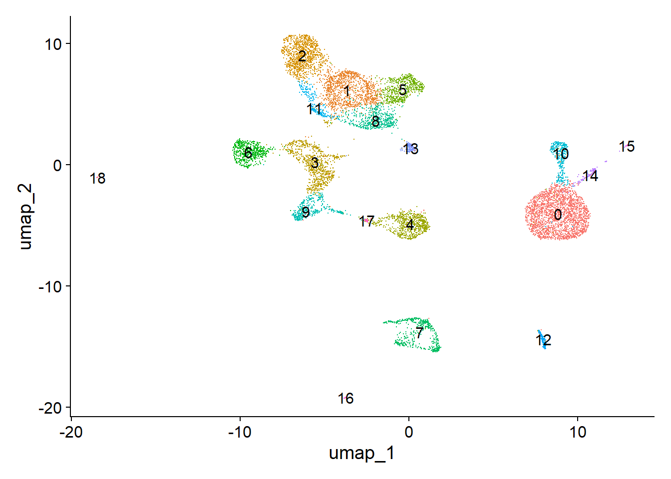
# load from Section 2 P14 - STEP: Find differentially accessible peaks between cell types, da_peaks
load(file = "data/pbmc.RData") # from Practical 13
# load(file = "data/pbmc_edited.RData")
# Idents(pbmc) <- pbmc$predicted.id
p1 <- DimPlot(pbmc, label = TRUE, pt.size = 0.1) + NoLegend()
p1

Code
# Get a list of motif position frequency matrices from the JASPAR database
pfm <- getMatrixSet(
    x = JASPAR2020,
    opts = list(species = "Homo sapiens", all_versions = FALSE)
)

# add motif information
pbmc <- AddMotifs(
  object = pbmc,
  genome = BSgenome.Hsapiens.UCSC.hg38,
  pfm = pfm
)
Building motif matrix
Finding motif positions
Creating Motif object

To facilitate motif analysis in Signac, we have created the Motif class to store all the required information, including a list of position weight matrices (PWMs) or position frequency matrices (PFMs) and a motif occurrence matrix. Here, the AddMotifs() function constructs a Motif object and adds it to our mouse brain dataset, along with other information such as the base composition of each peak. A motif object can be added to any Seurat assay using the SetAssayData() function. See the object interaction vignette for more information.

Cluster composition shows many clusters unique to the whole blood dataset:

Code
count_table <- table(pbmc@meta.data$seurat_clusters, pbmc@meta.data$orig.ident)
count_table
    
     SeuratProject
  0           2217
  1           1173
  2           1022
  3            877
  4            696
  5            615
  6            582
  7            510
  8            485
  9            397
  10           343
  11           234
  12           147
  13           127
  14           127
  15            30
  16            29
  17            29
  18             9

9.0.3 Step 2: Identifying enriched motifs / Finding overrepresented motifs

To identify potentially important cell-type-specific regulatory sequences, we can search for DNA motifs that are overrepresented in a set of peaks that are differentially accessible between cell types.

Here, we find differentially accessible peaks between Pvalb and Sst inhibitory interneurons. For sparse data (such as scATAC-seq), we find it is often necessary to lower the min.pct threshold in FindMarkers() from the default (0.1, which was designed for scRNA-seq data).

We then perform a hypergeometric test to test the probability of observing the motif at the given frequency by chance, comparing with a background set of peaks matched for GC content.

Code
# Find differentially accessible peaks in cluster 0 compared to cluster 1 (~1h 7m)
da_peaks <- FindMarkers(
    object = pbmc,
    #ident.1 = 'CD14+ Monocytes',
    #ident.2 = 'pre-B cell',
    ident.1 = '0',
    ident.2 = '1',
    only.pos = TRUE,
    min.pct = 0.05,
    test.use = 'LR',
    latent.vars = 'nCount_peaks'
)
Code
# Get the top differentially accessible peaks, with lowest p-values
top.da.peak <- rownames(da_peaks[da_peaks$p_val < 0.005 & da_peaks$pct.1 > 0.2, ])
Code
# save
save(da_peaks, file = "data/pbmc_markers.RData")
# save information
save(pbmc, top.da.peak, file = "data/pbmc_motifs.RData")
Code
load(file = "data/pbmc_motifs.RData")
# Find motifs enriched in these top differentially accessible peaks
enriched.motifs <- FindMotifs(
    object = pbmc,
    features = top.da.peak
)
Selecting background regions to match input sequence characteristics
Matching GC.percent distribution
Testing motif enrichment in 9842 regions
Code
head(enriched.motifs)
            motif observed background percent.observed percent.background
MA1513.1 MA1513.1     2242       4158         22.77992            10.3950
MA1653.1 MA1653.1     4400      12048         44.70636            30.1200
MA0599.1 MA0599.1     4388      12464         44.58443            31.1600
MA1650.1 MA1650.1     1336       2517         13.57448             6.2925
MA1564.1 MA1564.1     2822       7097         28.67303            17.7425
MA0162.4 MA0162.4     2380       5688         24.18208            14.2200
         fold.enrichment        pvalue motif.name      p.adjust
MA1513.1        2.191431  0.000000e+00      KLF15  0.000000e+00
MA1653.1        1.484275 1.089845e-276     ZNF148 3.449361e-274
MA0599.1        1.430823 1.261107e-231       KLF5 2.660937e-229
MA1650.1        2.157247 1.557382e-221     ZBTB14 2.464558e-219
MA1564.1        1.616065 1.728909e-216        SP9 2.188799e-214
MA0162.4        1.700568 5.025079e-212       EGR1 5.301458e-210
Code
MotifPlot(
  object = pbmc,
  motifs = head(rownames(enriched.motifs))
)
Warning: The `<scale>` argument of `guides()` cannot be `FALSE`. Use "none" instead as
of ggplot2 3.3.4.
ℹ The deprecated feature was likely used in the ggseqlogo package.
  Please report the issue at <https://github.com/omarwagih/ggseqlogo/issues>.

9.0.4 Step 3: Motif activity scores

We can also compute a per-cell motif activity score by running chromVAR. The motif activity score for a motif M is based on the number of reads mapping to peaks with motif M, after normalization correction for various biases: GC content, average number of reads mapping across all cells etc. You can read more about chromVar here. Motif activity scores allow us to visualize motif activities per cell.

Note

ChromVAR identifies motifs associated with variability in chromatin accessibility between cells. See the chromVAR paper for a complete description of the method.

It is also possible to directly test for differential activity scores between cell types, without looking at peaks with differential binding. This tends to give similar results as performing an enrichment test on differentially accessible peaks between the cell types (shown above).

Caution

This takes a while to run (around 5 minutes on Uppmax).

Code
# BiocManager::install("chromVAR")
library(chromVAR)
Code
# Use chromVAR to calculate the motif activities of all motifs in all cells.
chromvar_pbmc <- RunChromVAR(
    object = pbmc,
    genome = BSgenome.Hsapiens.UCSC.hg38,
    verbose = TRUE
)

DefaultAssay(chromvar_pbmc) <- 'chromvar'

# Look at results
pbmc$chromvar
GetAssayData(pbmc$chromvar)[1:10,1:3]
Code
# Have a look at the activitiy of the FOS motif, which has id MA0476.1
DefaultAssay(pbmc) <- 'chromvar'
FeaturePlot(
    object = pbmc,
    features = "MA0476.1",
    min.cutoff = 'q10',
    max.cutoff = 'q90',
    pt.size = 0.1
)
p1 + p2

We can also directly test for differential activity scores between cell types. This tends to give similar results as performing an enrichment test on differentially accessible peaks between the cell types (shown above).

When performing differential testing on the chromVAR z-score, we can set mean.fxn=rowMeans and fc.name="avg_diff" in the FindMarkers() function so that the fold-change calculation computes the average difference in z-score between the groups.

Code
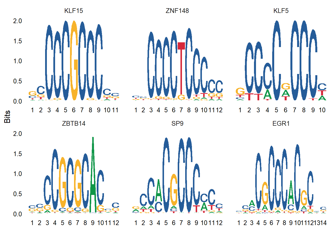
# Look for motifs that have differential activity between clusters 0 and 1.
differential.activity <- FindMarkers(
    object = pbmc,
    ident.1 = '0',
    ident.2 = '1',
    only.pos = TRUE,
    test.use = 'LR',
    min.pct = 0.2,
    latent.vars = 'nCount_peaks'
)

MotifPlot(
    object = pbmc,
    motifs = head(rownames(differential.activity)),
    assay = 'peaks'
)

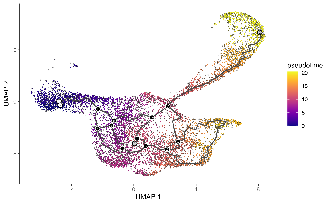
10 Building trajectories with Monocle 3

Also you can construct cell trajectories with Monocle 3 using single-cell ATAC-seq data. Please see the Monocle 3 website for information about installing Monocle 3.

11 Transcription factor footprinting

For this step we’ll use the dataset introduced and pre-processed in the trajectory building vignette.

Code
sessionInfo()
R version 4.4.1 (2024-06-14 ucrt)
Platform: x86_64-w64-mingw32/x64
Running under: Windows 11 x64 (build 22631)

Matrix products: default


locale:
[1] LC_COLLATE=English_United States.utf8 
[2] LC_CTYPE=English_United States.utf8   
[3] LC_MONETARY=English_United States.utf8
[4] LC_NUMERIC=C                          
[5] LC_TIME=English_United States.utf8    

time zone: America/Mexico_City
tzcode source: internal

attached base packages:
[1] stats4    stats     graphics  grDevices utils     datasets  methods  
[8] base     

other attached packages:
 [1] chromVAR_1.26.0                   ggseqlogo_0.2                    
 [3] motifmatchr_1.26.0                patchwork_1.3.0.9000             
 [5] BSgenome.Hsapiens.UCSC.hg38_1.4.5 BSgenome_1.72.0                  
 [7] rtracklayer_1.64.0                BiocIO_1.14.0                    
 [9] Biostrings_2.72.1                 XVector_0.44.0                   
[11] GenomicRanges_1.56.2              GenomeInfoDb_1.40.1              
[13] IRanges_2.38.1                    S4Vectors_0.42.1                 
[15] BiocGenerics_0.50.0               TFBSTools_1.42.0                 
[17] JASPAR2020_0.99.10                Seurat_5.1.0                     
[19] SeuratObject_5.0.2                sp_2.1-4                         
[21] Signac_1.14.0                    

loaded via a namespace (and not attached):
  [1] RcppAnnoy_0.0.22            splines_4.4.1              
  [3] later_1.3.2                 bitops_1.0-8               
  [5] R.oo_1.26.0                 tibble_3.2.1               
  [7] polyclip_1.10-7             XML_3.99-0.17              
  [9] DirichletMultinomial_1.46.0 fastDummies_1.7.4          
 [11] lifecycle_1.0.4             pwalign_1.0.0              
 [13] globals_0.16.3              lattice_0.22-6             
 [15] MASS_7.3-60.2               magrittr_2.0.3             
 [17] plotly_4.10.4               rmarkdown_2.28             
 [19] yaml_2.3.10                 httpuv_1.6.15              
 [21] sctransform_0.4.1           spam_2.10-0                
 [23] spatstat.sparse_3.1-0       reticulate_1.39.0          
 [25] cowplot_1.1.3               pbapply_1.7-2              
 [27] DBI_1.2.3                   CNEr_1.40.0                
 [29] RColorBrewer_1.1-3          abind_1.4-8                
 [31] zlibbioc_1.50.0             Rtsne_0.17                 
 [33] R.utils_2.12.3              purrr_1.0.2                
 [35] RCurl_1.98-1.16             pracma_2.4.4               
 [37] GenomeInfoDbData_1.2.12     ggrepel_0.9.6              
 [39] irlba_2.3.5.1               listenv_0.9.1              
 [41] spatstat.utils_3.1-0        seqLogo_1.70.0             
 [43] goftest_1.2-3               RSpectra_0.16-2            
 [45] annotate_1.82.0             spatstat.random_3.3-2      
 [47] fitdistrplus_1.2-1          parallelly_1.38.0          
 [49] leiden_0.4.3.1              codetools_0.2-20           
 [51] DelayedArray_0.30.1         RcppRoll_0.3.1             
 [53] DT_0.33                     tidyselect_1.2.1           
 [55] UCSC.utils_1.0.0            farver_2.1.2               
 [57] matrixStats_1.4.0           spatstat.explore_3.3-2     
 [59] GenomicAlignments_1.40.0    jsonlite_1.8.8             
 [61] progressr_0.14.0            ggridges_0.5.6             
 [63] survival_3.6-4              tools_4.4.1                
 [65] TFMPvalue_0.0.9             ica_1.0-3                  
 [67] Rcpp_1.0.13                 glue_1.7.0                 
 [69] gridExtra_2.3               SparseArray_1.4.8          
 [71] xfun_0.48                   MatrixGenerics_1.16.0      
 [73] dplyr_1.1.4                 withr_3.0.1                
 [75] fastmap_1.2.0               fansi_1.0.6                
 [77] caTools_1.18.3              digest_0.6.36              
 [79] R6_2.5.1                    mime_0.12                  
 [81] colorspace_2.1-1            GO.db_3.19.1               
 [83] scattermore_1.2             poweRlaw_0.80.0            
 [85] gtools_3.9.5                tensor_1.5                 
 [87] spatstat.data_3.1-2         RSQLite_2.3.7              
 [89] R.methodsS3_1.8.2           utf8_1.2.4                 
 [91] tidyr_1.3.1                 generics_0.1.3             
 [93] data.table_1.16.2           httr_1.4.7                 
 [95] htmlwidgets_1.6.4           S4Arrays_1.4.1             
 [97] uwot_0.2.2                  pkgconfig_2.0.3            
 [99] gtable_0.3.5                blob_1.2.4                 
[101] lmtest_0.9-40               htmltools_0.5.8.1          
[103] dotCall64_1.1-1             scales_1.3.0               
[105] Biobase_2.64.0              png_0.1-8                  
[107] spatstat.univar_3.0-1       knitr_1.48                 
[109] rstudioapi_0.17.0           tzdb_0.4.0                 
[111] rjson_0.2.23                reshape2_1.4.4             
[113] curl_5.2.3                  nlme_3.1-164               
[115] zoo_1.8-12                  cachem_1.1.0               
[117] stringr_1.5.1               KernSmooth_2.23-24         
[119] parallel_4.4.1              miniUI_0.1.1.1             
[121] AnnotationDbi_1.66.0        restfulr_0.0.15            
[123] pillar_1.9.0                grid_4.4.1                 
[125] vctrs_0.6.5                 RANN_2.6.2                 
[127] promises_1.3.0              xtable_1.8-4               
[129] cluster_2.1.6               evaluate_1.0.1             
[131] readr_2.1.5                 cli_3.6.2                  
[133] compiler_4.4.1              Rsamtools_2.20.0           
[135] rlang_1.1.3                 crayon_1.5.3               
[137] future.apply_1.11.2         labeling_0.4.3             
[139] plyr_1.8.9                  stringi_1.8.4              
[141] viridisLite_0.4.2           deldir_2.0-4               
[143] BiocParallel_1.38.0         munsell_0.5.1              
[145] lazyeval_0.2.2              spatstat.geom_3.3-3        
[147] Matrix_1.7-0                RcppHNSW_0.6.0             
[149] hms_1.1.3                   bit64_4.5.2                
[151] future_1.34.0               ggplot2_3.5.1              
[153] KEGGREST_1.44.1             shiny_1.9.1                
[155] SummarizedExperiment_1.34.0 ROCR_1.0-11                
[157] igraph_2.0.3                memoise_2.0.1              
[159] fastmatch_1.1-4             bit_4.5.0                  

11.1 References