Lesson 4: Biological functions of differentially expressed genes

Welcome

In the previous lesson we found 94 differentially expressed genes (DEGs) between lupus patients and controls. A list of genes, on its own, says little: the question now is what do these genes do, and do they take part in common biological processes?

What you need to know beforehand: you should have completed the lesson Differentially expressed genes between patients and controls.

By the end you will be able to:

Explain what a functional enrichment analysis is and what question it answers.
Run an enrichment analysis with g:Profiler and interpret its results.
Recognize the main functional databases (Gene Ontology, Reactome, KEGG…).
Identify lupus-associated genes and interferon-stimulated genes among the DEGs.
Reproduce Figure 3 of the article.
Correlate ISG expression with disease activity (SLEDAI).

Estimated time: 1.5 hours.

Lesson map

flowchart LR
  A["de_results
(lesson 3)"] --> B["94 DEGs by cell
type and direction"]
  B --> C["g:Profiler:
enrichment"]
  B --> D["Reference lists:
SLE and ISG"]
  C --> E["3A. DEG heatmaps,
LFC and annotations"]
  D --> F["3B and 3C. Dot plots"]
  C --> G["3D. REAC and BP processes"]
  E --> H["Figure 3"]
  F --> H
  G --> H
  D --> I["ISG vs SLEDAI:
Spearman"]

Glossary

These are the terms we will use. Come back here whenever you need to.

Functional annotation: information about what a gene does (processes, pathways, localization…).
Term: a functional category, for example “response to virus”, with its list of genes.
Functional enrichment: tests whether a term appears in our gene list more often than expected by chance.
Hypergeometric test: the statistical test behind enrichment (like drawing marbles from a bag without replacement).
Gene Ontology (GO): a vocabulary of functions with three branches: biological process (BP), cellular component (CC), and molecular function (MF).
Reactome (REAC), KEGG, WikiPathways (WP): databases of biological pathways.
TF: transcription factor binding sites. MIRNA: microRNA targets. HP: human phenotypes. CORUM: protein complexes.
Parent / specific term: databases are organized in hierarchies; a general (parent) term contains more specific terms.
ISG (interferon-stimulated genes): genes that are switched on in response to interferon.
SLEDAI (SLE Disease Activity Index): lupus activity score; higher = more active disease.
Spearman correlation (rho): measures whether two variables go up or down together by comparing their ranks; it ranges from −1 to 1.

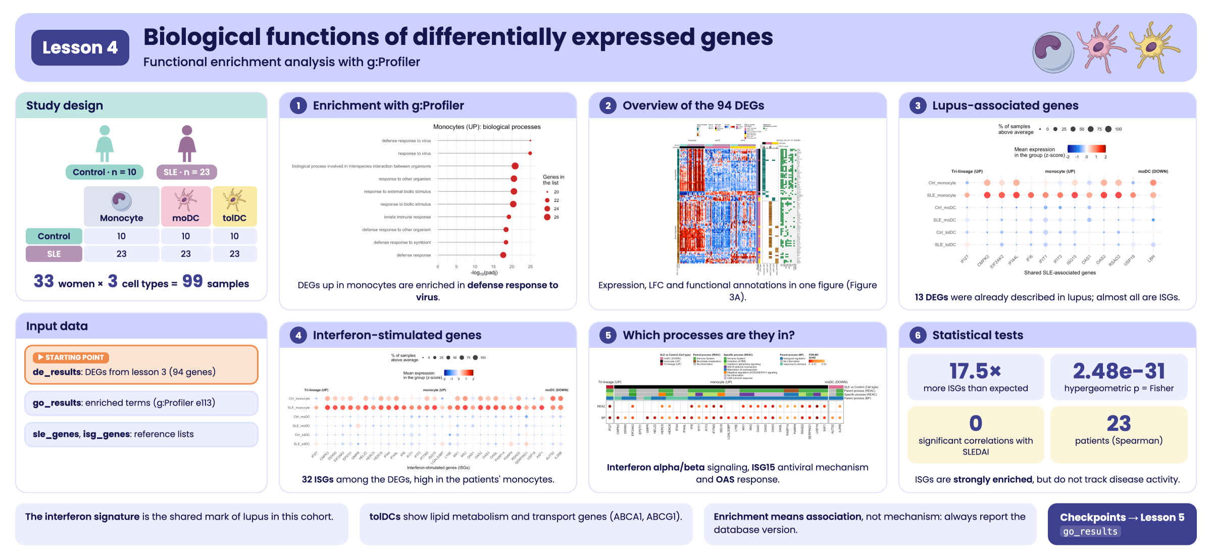
Visual summary of lesson 4.

1. Setup

library(GeneExprLupusMx) # package data
library(tidyverse)       # table manipulation and plots
library(ComplexHeatmap)  # heatmaps
library(circlize)        # color scales for ComplexHeatmap
library(grid)            # drawing shapes inside the heatmaps
library(cowplot)         # combining plots into a panel

# Large package objects: downloaded only the first time (see ?download_data)
zscore_mat <- download_data("zscore_mat")

Colors and thresholds (the same as in the previous lesson):

cell_color  <- c(monocyte = "black", moDC = "palevioletred", tolDC = "gold1")
group_color <- c(Ctrl = "#96d4ccff", SLE = "#b493b4ff")

lfc_threshold  <- 1
padj_threshold <- 0.05

Starting point: the DEGs from the previous lesson

The de_results checkpoint contains the DESeq2 results for the three cell types. We gather the DEGs into a single table:

deg_df <- bind_rows(lapply(names(de_results), function(cell) {
  de_results[[cell]] %>%
    filter(!is.na(padj), padj < padj_threshold, abs(log2FoldChange) >= lfc_threshold) %>%
    mutate(Cell_type  = cell,
           Expression = ifelse(log2FoldChange > 0, "Up-regulated", "Down-regulated"),
           query      = paste("SLE", ifelse(log2FoldChange > 0, "UP", "DOWN"), cell, sep = "_"))
}))

dplyr::count(deg_df, query)
#>             query  n
#> 1   SLE_DOWN_moDC 40
#> 2  SLE_DOWN_tolDC 12
#> 3     SLE_UP_moDC  4
#> 4 SLE_UP_monocyte 37
#> 5    SLE_UP_tolDC  4

Each combination of cell type and direction is a gene list (query). Monocytes have no down-regulated genes, so there are five lists.

The same gene can be a DEG in more than one cell type. For the plots we need one row per gene (94 genes) and a label describing its pattern: in which cell types it changes.

genes_in <- function(cell, direction) {
  deg_df$gene[deg_df$Cell_type == cell & deg_df$Expression == direction]
}

gene_info <- deg_df %>%
  distinct(gene, .keep_all = TRUE) %>% # one row per gene
  mutate(pattern = case_when(
    gene %in% Reduce(intersect, list(genes_in("monocyte", "Up-regulated"),
                                     genes_in("moDC", "Up-regulated"),
                                     genes_in("tolDC", "Up-regulated"))) ~ "Tri-lineage (UP)",
    gene %in% intersect(genes_in("moDC", "Down-regulated"),
                        genes_in("tolDC", "Down-regulated")) ~ "moDC & tolDC (DOWN)",
    gene %in% genes_in("monocyte", "Up-regulated") ~ "monocyte (UP)",
    gene %in% genes_in("moDC", "Up-regulated")     ~ "moDC (UP)",
    gene %in% genes_in("moDC", "Down-regulated")   ~ "moDC (DOWN)",
    gene %in% genes_in("tolDC", "Up-regulated")    ~ "tolDC (UP)",
    gene %in% genes_in("tolDC", "Down-regulated")  ~ "tolDC (DOWN)"))

dplyr::count(gene_info, pattern)
#>               pattern  n
#> 1    Tri-lineage (UP)  1
#> 2 moDC & tolDC (DOWN)  1
#> 3         moDC (DOWN) 39
#> 4           moDC (UP)  3
#> 5       monocyte (UP) 36
#> 6        tolDC (DOWN) 11
#> 7          tolDC (UP)  3

Tri-lineage (UP) are the genes that go up in all three cell types (only IFI27), and moDC & tolDC (DOWN) are those that go down in both dendritic cell types.

2. What is an enrichment analysis?

Imagine a bag with 20,000 marbles (all the genes in the genome). 200 of them are red: the genes of a term, for example “response to virus”. We draw 37 marbles at random (our monocyte DEGs). We would expect to draw fewer than one red marble. If we draw 15, something is not down to chance: our genes are enriched in that term.

The hypergeometric test calculates how likely it is to draw that many red marbles by chance. Because thousands of terms are tested at once, the p-values are corrected (FDR), just as in differential expression.

Enrichment is not causation. A list being enriched in “response to virus” does not mean there is a virus: it means the genes that change tend to take part together in that function. It is a clue for generating hypotheses.

3. Step 1: enrichment with g:Profiler

g:Profiler queries several databases at the same time (GO, Reactome, KEGG, WikiPathways, TF, miRNA, HP, CORUM). In R it is used through the gost() function of the gprofiler2 package:

library(gprofiler2)

deg_lists <- split(deg_df$gene, deg_df$query) # one gene list per query

# Archived version of g:Profiler (June 2025)
set_base_url("https://biit.cs.ut.ee/gprofiler_archive3/e113_eg59_p19")

gost_res <- gost(deg_lists,
                 organism          = "hsapiens", # human
                 correction_method = "fdr",      # multiple-testing correction
                 user_threshold    = 0.05,       # maximum padj
                 evcodes           = TRUE)       # include which genes each term has

Databases change. g:Profiler updates its annotations several times a year, so the same gene list can give somewhat different results over time. To make your analyses reproducible, pin the version with set_base_url() and report it.

gost() needs an internet connection. So that this lesson works offline, the package includes the result as a checkpoint, go_results:

attr(go_results, "gprofiler_version")
#> [1] "e113_eg59_p19_903d2221"
glimpse(go_results)
#> Rows: 943
#> Columns: 10
#> $ query             <chr> "SLE_DOWN_moDC", "SLE_DOWN_moDC", "SLE_DOWN_moDC", "…
#> $ source            <chr> "CORUM", "CORUM", "CORUM", "CORUM", "CORUM", "CORUM"…
#> $ term_id           <chr> "CORUM:7577", "CORUM:6805", "CORUM:6799", "CORUM:679…
#> $ term_name         <chr> "APP-APBB1-KAT5 complex", "S1PR1-beta-arrestin 2 com…
#> $ term_size         <int> 3, 2, 3, 2, 3, 2, 3, 3, 2, 3, 2, 3, 3, 3, 4, 4, 560,…
#> $ query_size        <int> 7, 7, 7, 7, 7, 7, 7, 7, 7, 7, 7, 7, 7, 7, 7, 7, 36, …
#> $ intersection_size <int> 1, 1, 1, 1, 1, 1, 1, 1, 1, 1, 1, 1, 1, 1, 1, 1, 10, …
#> $ p_value           <dbl> 7.524322e-03, 7.524322e-03, 7.524322e-03, 7.524322e-…
#> $ parents           <chr> "CORUM:0000000", "CORUM:0000000", "CORUM:0000000", "…
#> $ intersection      <chr> "APBB1", "S1PR1", "S1PR1", "S1PR1", "APBB1", "HIP1R"…

The most important columns are:

Column	Meaning
`query`	Gene list (cell type and direction)
`source`	Database
`term_name`	Term name
`term_size`	Genes annotated to the term in the whole genome
`intersection_size`	Genes from our list annotated to the term
`p_value`	Adjusted p-value (FDR)
`intersection`	Which genes those are

How many significant terms are there per list and database?

go_results %>%
  dplyr::count(query, source) %>%
  pivot_wider(names_from = source, values_from = n, values_fill = 0)
#> # A tibble: 5 × 11
#>   query        CORUM `GO:BP` `GO:CC`    HP  KEGG  REAC    WP `GO:MF` MIRNA    TF
#>   <chr>        <int>   <int>   <int> <int> <int> <int> <int>   <int> <int> <int>
#> 1 SLE_DOWN_mo…    16     201       7    48    10     1     8       0     0     0
#> 2 SLE_DOWN_to…     6       0       0     3     0    10    12       8     0     0
#> 3 SLE_UP_moDC      0       0       0     0     1     1     3       4     0     0
#> 4 SLE_UP_mono…     2     183       2     0    10    19    12      15     1    78
#> 5 SLE_UP_tolDC     0     172       6    14     5    16    16      53     0     0

The lists with the most genes (monocytes UP, moDC DOWN) have more terms, and most come from GO:BP, the largest database.

3.1 The most significant terms

Let us look at the 10 most significant biological processes (GO:BP) in monocytes:

go_results %>%
  filter(query == "SLE_UP_monocyte", source == "GO:BP") %>%
  slice_min(p_value, n = 10, with_ties = FALSE) %>%
  ggplot(aes(x = -log10(p_value), y = reorder(term_name, -log10(p_value)))) +
  geom_segment(aes(x = 0, xend = -log10(p_value), yend = term_name), color = "grey60") +
  geom_point(aes(size = intersection_size), color = "firebrick3") +
  labs(x = expression("-log"[10] * "(padj)"), y = NULL, size = "Genes in\nthe list",
       title = "Monocytes (UP): biological processes") +
  theme_minimal()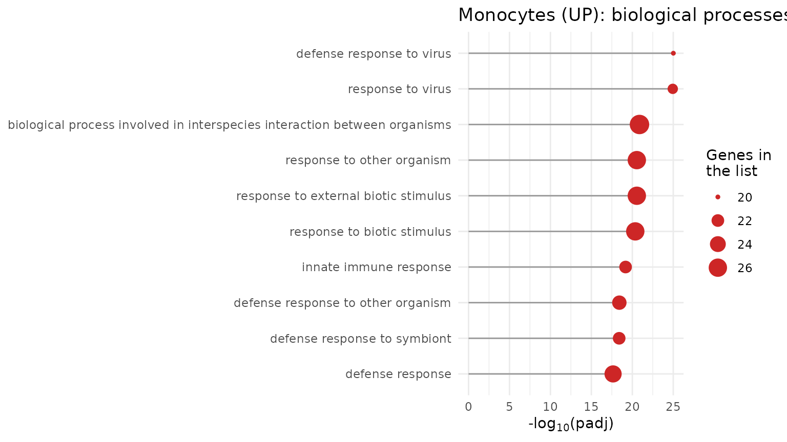

All the terms have to do with the response to viruses and to interferon: the interferon signature we saw in the previous lessons, now backed by the enrichment analysis.

Challenge 1. What are the 5 most significant Reactome (REAC) terms in tolDCs with up-regulated genes (SLE_UP_tolDC)? What kind of processes are they?

Show solution

go_results %>%
  filter(query == "SLE_UP_tolDC", source == "REAC") %>%
  slice_min(p_value, n = 5, with_ties = FALSE) %>%
  dplyr::select(term_name, intersection_size, p_value, intersection)
#>                                                                           term_name
#> 1 NR1H3 & NR1H2 regulate gene expression linked to cholesterol transport and efflux
#> 2                                                NR1H2 and NR1H3-mediated signaling
#> 3                            Plasma lipoprotein assembly, remodeling, and clearance
#> 4                                                        Defective ABCA1 causes TGD
#> 5                                                                      HDL assembly
#>   intersection_size      p_value intersection
#> 1                 2 0.0006116482  ABCA1,ABCG1
#> 2                 2 0.0006116482  ABCA1,ABCG1
#> 3                 2 0.0010219157  ABCA1,ABCG1
#> 4                 1 0.0034075420        ABCA1
#> 5                 1 0.0084434412        ABCA1

These are processes of lipid and cholesterol metabolism and transport (for example, the ABCA1 pathway), very different from the interferon response seen in monocytes.

4. Step 2: overview of the 94 DEGs (Figure 3A)

We will build three heatmaps aligned by gene:

Expression (z-score) of each DEG across all samples.
LFC of each gene in each DEG list.
Presence of significant annotation in each database.

4.1 Expression heatmap

We order the samples by cell type and group, and take the z-scores of the 94 genes from the zscore_mat checkpoint:

sample_order <- metadata_cleaned %>%
  mutate(Cell_type = factor(Cell_type, levels = c("monocyte", "moDC", "tolDC"))) %>%
  arrange(Cell_type, Group)

deg_mat <- zscore_mat[gene_info$gene, sample_order$sample_ID]
dim(deg_mat)
#> [1] 94 99

We add annotations: on top, the group and cell type of each sample; on the left, the LFC; on the right, the gene biotype (from biotype_summary) and its pattern.

pattern_color <- c("Tri-lineage (UP)" = "#b2182b", "monocyte (UP)" = "black",
                   "moDC (UP)" = "palevioletred", "moDC (DOWN)" = "palevioletred",
                   "tolDC (UP)" = "gold1", "tolDC (DOWN)" = "gold1",
                   "moDC & tolDC (DOWN)" = "blue")
biotype_color <- c("PCG" = "#7570B3", "lncRNA" = "#E7298A")
lfc_color <- colorRamp2(c(-2, -1, 0, 1, 2), c("#8c510a", "#bf812d", "white", "#35978f", "#01665e"))
zscore_color <- colorRamp2(c(-2, -1, 0, 1, 2), c("darkblue", "dodgerblue", "white", "red", "darkred"))

gene_biotype <- biotype_summary$Group_biotype[match(gene_info$gene, biotype_summary$gene)]
table(gene_biotype)
#> gene_biotype
#> lncRNA    PCG 
#>      4     90

sample_anno <- HeatmapAnnotation(
  Group       = as.character(sample_order$Group),
  "Cell type" = as.character(sample_order$Cell_type),
  col = list(Group = group_color, "Cell type" = cell_color),
  annotation_name_side = "left")

ht_expression <- Heatmap(
  deg_mat, name = "Z-score", col = zscore_color,
  cluster_rows = TRUE, cluster_columns = FALSE, show_row_dend = FALSE,
  show_row_names = FALSE, show_column_names = FALSE,
  top_annotation  = sample_anno,
  left_annotation = rowAnnotation("SLE vs Control\n(LFC)" = gene_info$log2FoldChange,
                                  col = list("SLE vs Control\n(LFC)" = lfc_color)),
  right_annotation = rowAnnotation(Biotype = gene_biotype,
                                   "SLE vs Control\n(Cell type)" = gene_info$pattern,
                                   col = list(Biotype = biotype_color,
                                              "SLE vs Control\n(Cell type)" = pattern_color)),
  column_split = sample_order$Cell_type,
  row_split    = factor(gene_info$Expression, levels = c("Up-regulated", "Down-regulated")),
  heatmap_legend_param = list(direction = "horizontal"))

4.2 LFC heatmap by list

A matrix with the LFC of each gene in each DEG list (0 if the gene is not a DEG in that list). On top, a barplot with the number of DEGs in each list:

lfc_mat <- deg_df %>%
  mutate(column = str_replace(query, "SLE_(UP|DOWN)_(.*)", "\\2 (\\1)")) %>% # "monocyte (UP)"
  dplyr::select(gene, column, log2FoldChange) %>%
  pivot_wider(names_from = column, values_from = log2FoldChange, values_fill = 0) %>%
  column_to_rownames("gene") %>%
  as.matrix()
lfc_mat <- lfc_mat[gene_info$gene, c("monocyte (UP)", "moDC (UP)", "moDC (DOWN)",
                                     "tolDC (UP)", "tolDC (DOWN)")]
colSums(lfc_mat != 0)
#> monocyte (UP)     moDC (UP)   moDC (DOWN)    tolDC (UP)  tolDC (DOWN) 
#>            37             4            40             4            12

ht_lfc <- Heatmap(
  lfc_mat, name = "SLE vs Control\n(LFC)", col = lfc_color, show_heatmap_legend = FALSE,
  cluster_columns = FALSE, show_row_names = FALSE,
  rect_gp = gpar(col = "#f0f0f0", lwd = 1), border = TRUE,
  top_annotation = HeatmapAnnotation(
    "Cell type"  = c("monocyte", "moDC", "moDC", "tolDC", "tolDC"),
    "DEG Counts" = anno_barplot(colSums(lfc_mat != 0), add_numbers = TRUE, height = unit(1, "cm")),
    col = list("Cell type" = cell_color), show_legend = FALSE),
  width = unit(4, "cm"))

4.3 Annotation heatmap

In which databases does each gene have at least one significant term? We split the intersection column (comma-separated genes) into one row per gene:

gene_source <- go_results %>%
  dplyr::select(source, intersection) %>%
  separate_rows(intersection, sep = ",") %>%
  distinct(gene = intersection, source = str_remove(source, "GO:"))

presence_mat <- gene_source %>%
  mutate(present = "yes") %>%
  pivot_wider(names_from = source, values_from = present, values_fill = "no") %>%
  right_join(tibble(gene = gene_info$gene), by = "gene") %>% # the 94 DEGs
  mutate(across(-gene, ~ replace_na(.x, "no"))) %>%
  column_to_rownames("gene") %>%
  as.matrix()
presence_mat <- presence_mat[gene_info$gene,
                             c("BP", "CC", "MF", "REAC", "HP", "KEGG", "WP", "TF", "CORUM", "MIRNA")]
colSums(presence_mat == "yes")
#>    BP    CC    MF  REAC    HP  KEGG    WP    TF CORUM MIRNA 
#>    70    63    19    43    17    22    31    31    10    12

n_up   <- sum(gene_info$Expression == "Up-regulated")
n_down <- sum(gene_info$Expression == "Down-regulated")

ht_presence <- Heatmap(
  presence_mat, name = "Significant\nannotation presence",
  col = c(yes = "#238b45", no = "#f0f0f0"),
  cluster_columns = FALSE, show_row_names = TRUE, row_names_gp = gpar(fontsize = 7),
  rect_gp = gpar(col = "white", lwd = 1),
  column_title = paste0(nrow(gene_info), " DEG (", n_up, " UP / ", n_down, " DOWN)"),
  width = unit(4, "cm"))

4.4 All three together

When joining heatmaps with +, ComplexHeatmap applies the row order of the first one to all of them, so each row is the same gene in all three:

ht_fig3a <- ht_expression + ht_lfc + ht_presence

ht_opt$message <- FALSE
draw(ht_fig3a, ht_gap = unit(5, "mm"), merge_legends = TRUE,
     heatmap_legend_side = "top", annotation_legend_side = "top")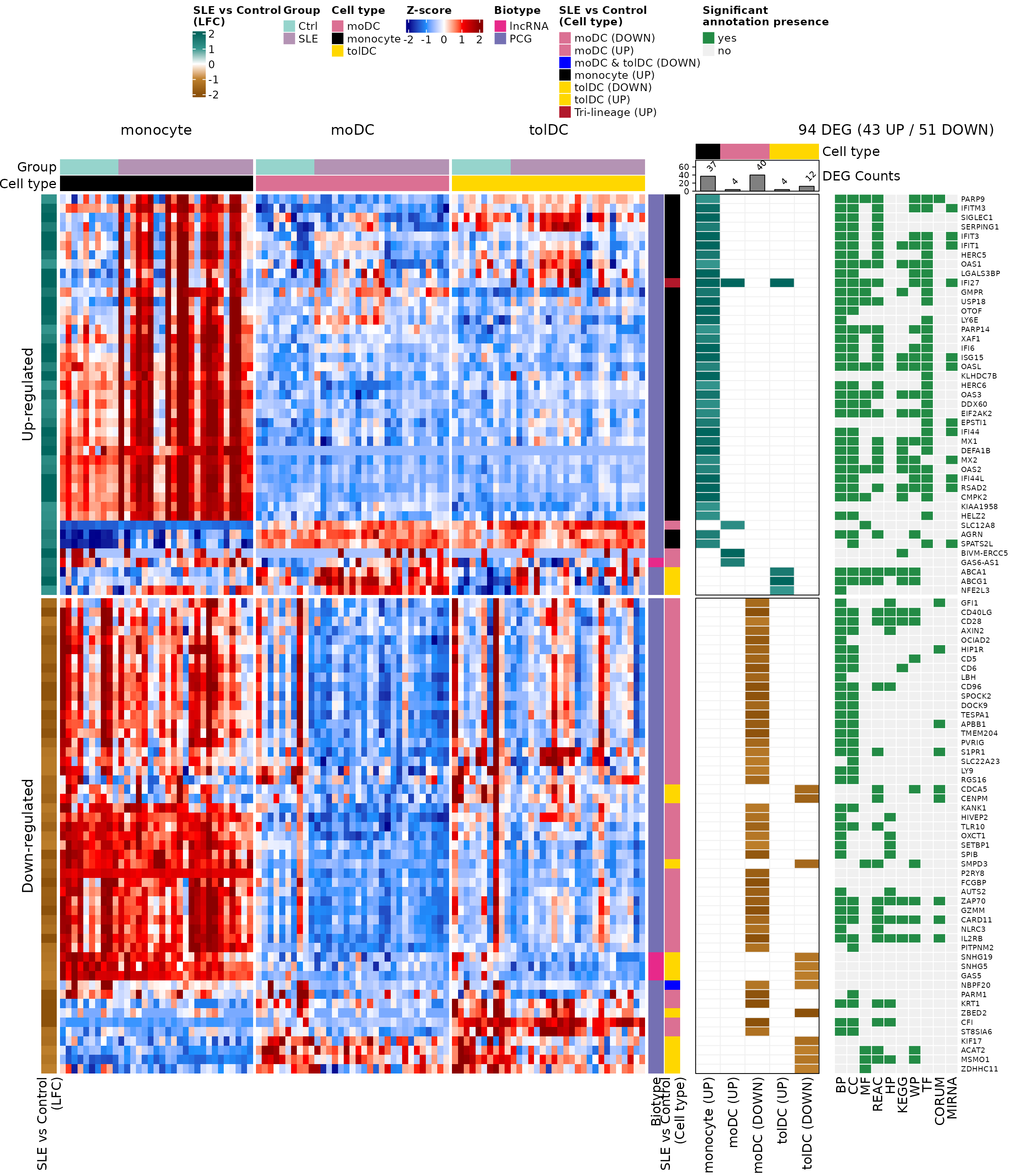

What do you observe?

The genes that go up (top block) are mostly monocyte genes and have many annotations in almost all databases: they are well-studied immune response genes.
The genes that go down are mostly moDC genes; several have few annotations or none, including the lncRNAs.
In the expression column, the patients’ monocyte block stands out in red for the up-regulated genes: this is the interferon signature.

5. Step 3: lupus-associated genes and ISGs (Figures 3B and 3C)

We compare the DEGs with two reference lists included in the package:

sle_genes: genes associated with lupus in the literature (four studies).
isg_genes: 423 interferon-stimulated genes (Yu et al., 2025).

sle_deg <- intersect(unique(sle_genes$Gene_name), gene_info$gene)
isg_deg <- intersect(isg_genes$genes, gene_info$gene)
sle_deg
#>  [1] "IFI44L"  "RSAD2"   "USP18"   "IFIT3"   "CMPK2"   "ISG15"   "IFI6"   
#>  [8] "IFI27"   "IFIT1"   "LBH"     "OAS1"    "OAS2"    "EIF2AK2"
length(isg_deg)
#> [1] 32

13 DEGs were already associated with lupus and 32 are ISGs. We plot them as in the previous lesson: a dot plot with the mean expression (z-score) by group and cell type. Since we will do this twice, we save it in a function:

plot_gene_dots <- function(genes, x_label, gene_levels = sort(genes)) {
  dots_df <- as.data.frame(zscore_mat[genes, ]) %>%
    rownames_to_column("gene") %>%
    pivot_longer(-gene, names_to = "sample_ID", values_to = "expression") %>%
    left_join(dplyr::select(metadata_cleaned, sample_ID, Group, Cell_type), by = "sample_ID") %>%
    group_by(Group, Cell_type, gene) %>%
    summarise(mean_expression = mean(expression),
              pct_expressed   = 100 * mean(expression > 0), .groups = "drop") %>%
    left_join(dplyr::select(gene_info, gene, pattern), by = "gene") %>%
    mutate(condition = factor(paste(Group, Cell_type, sep = "_"),
                              levels = c("SLE_tolDC", "Ctrl_tolDC", "SLE_moDC",
                                         "Ctrl_moDC", "SLE_monocyte", "Ctrl_monocyte")),
           pattern = factor(pattern, levels = c("Tri-lineage (UP)", "monocyte (UP)", "moDC (DOWN)")),
           gene    = factor(gene, levels = gene_levels))

  min_val <- min(dots_df$mean_expression)
  max_val <- max(dots_df$mean_expression)

  ggplot(dots_df, aes(x = gene, y = condition, color = mean_expression, size = pct_expressed)) +
    geom_point(alpha = 0.8) +
    scale_color_gradientn(colors = c("darkblue", "dodgerblue", "white", "red", "darkred"),
                          values = scales::rescale(c(-2, min_val, 0, max_val, 2)),
                          limits = c(-2, 2), oob = scales::squish) +
    ggh4x::facet_grid2(~ pattern, scales = "free_x", space = "free_x",
                       strip = ggh4x::strip_vanilla(clip = "off")) +
    labs(x = x_label, y = NULL,
         color = "Mean expression\nin the group (z-score)",
         size = "% of samples\nabove average") +
    theme_minimal(base_size = 12) +
    theme(legend.position = "top", legend.box = "vertical",
          strip.text.x = element_text(face = "bold"),
          axis.text.x = element_text(angle = 45, hjust = 1),
          plot.margin = margin(5.5, 40, 5.5, 5.5)) # margin so the last label is not cut off
}

p_sle <- plot_gene_dots(sle_deg, "Shared SLE-associated genes",
                        gene_levels = c("IFI27", "CMPK2", "EIF2AK2", "IFI44L", "IFI6", "IFIT1",
                                        "IFIT3", "ISG15", "OAS1", "OAS2", "RSAD2", "USP18", "LBH"))
p_sle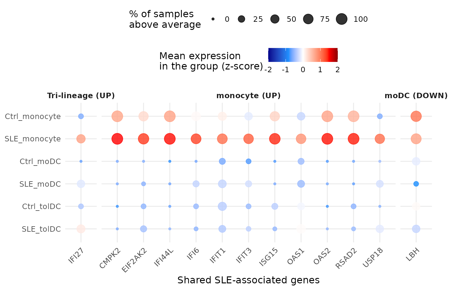

p_isg <- plot_gene_dots(isg_deg, "Interferon-stimulated genes (ISGs)")
p_isg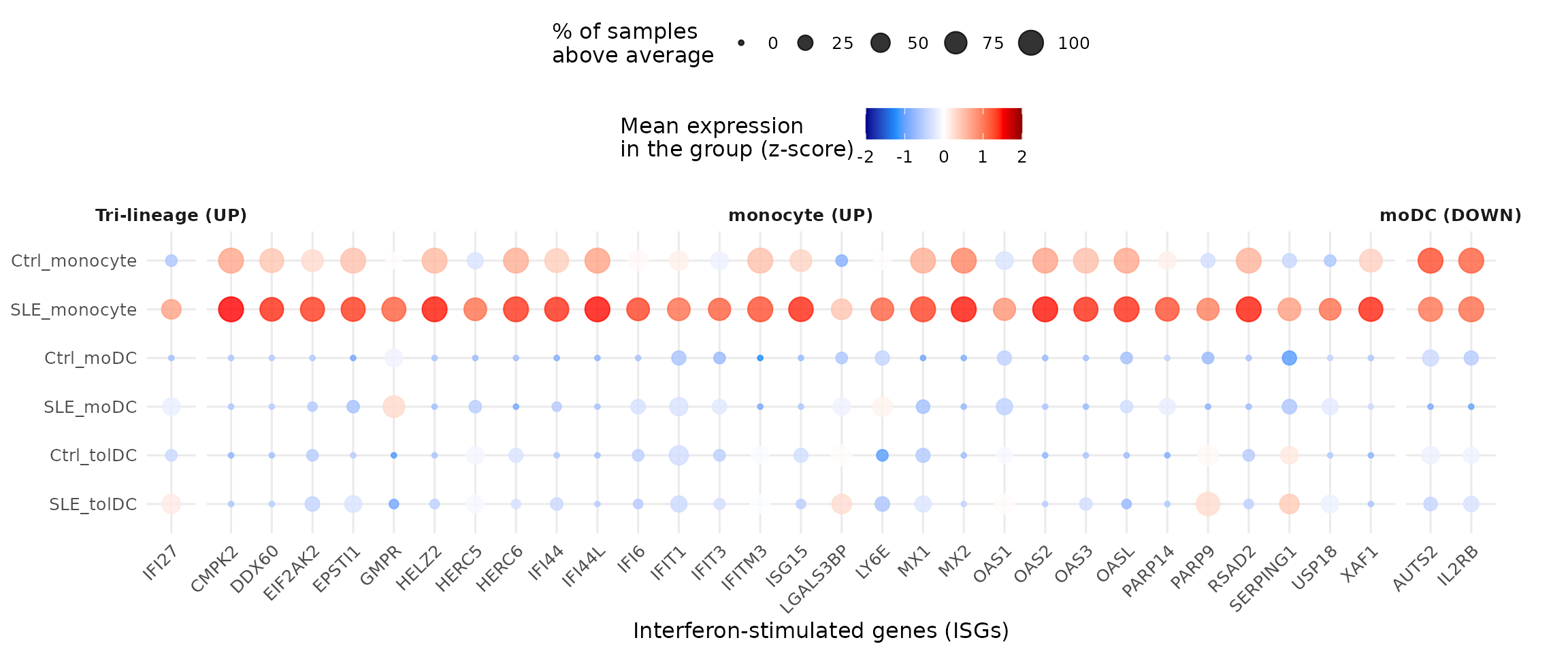

Almost all the lupus-associated genes we found are also ISGs, and they are highest in the patients’ monocytes (row SLE_monocyte). IFI27 is the exception that proves the rule: it goes up in all three cell types. In contrast, LBH, AUTS2, and IL2RB are DEGs that go down in the patients’ moDCs. In the plot they stand out more for their high expression in monocytes, because the z-score compares each sample with all the others, across the three cell types.

5.1 Are there more ISGs than expected by chance?

32 of the 94 DEGs are ISGs. Is that a lot? We answer with the hypergeometric test from section 2: if we draw 94 marbles (DEGs) from a bag with all the genes in the package, how likely is it that 32 or more are red (ISGs)?

We need four numbers:

N <- nrow(de_results$monocyte) # universe: all genes in the package
m <- nrow(isg_genes)           # ISGs in the reference list
k <- nrow(gene_info)           # DEGs
q <- length(isg_deg)           # DEGs that are ISGs

c(N = N, m = m, k = k, q = q)
#>     N     m     k     q 
#> 21718   423    94    32
k * m / N # ISGs expected among the DEGs by chance
#> [1] 1.830832

By chance we would expect fewer than 2 ISGs among the DEGs, and we found 32: a 17.5-fold enrichment.

phyper() gives the probability of drawing more than q - 1 red marbles, that is, q or more. We use lower.tail = FALSE because we care about the upper tail (over-representation):

p_hyper <- phyper(q - 1, m, N - m, k, lower.tail = FALSE)
p_hyper
#> [1] 2.484086e-31

Fisher’s exact test asks the same question with a 2 × 2 table. With the one-sided alternative ("greater") it is exactly the same test:

isg_table <- matrix(c(q, k - q, m - q, N - m - k + q), nrow = 2,
                    dimnames = list(ISG = c("Yes", "No"), DEG = c("Yes", "No")))
isg_table
#>      DEG
#> ISG   Yes    No
#>   Yes  32   391
#>   No   62 21233

isg_fisher <- fisher.test(isg_table, alternative = "greater")
isg_fisher
#> 
#>  Fisher's Exact Test for Count Data
#> 
#> data:  isg_table
#> p-value < 2.2e-16
#> alternative hypothesis: true odds ratio is greater than 1
#> 95 percent confidence interval:
#>  18.80807      Inf
#> sample estimates:
#> odds ratio 
#>   27.98511
isg_fisher$p.value
#> [1] 2.484086e-31

When printing the result, R shows p-value < 2.2e-16: that is the limit it uses to display p-values, not the actual value. The full value is in isg_fisher$p.value and matches phyper(): 2.48e-31. Both tests reach the same conclusion: ISGs are strongly enriched among the DEGs (odds ratio = 28).

Challenge 2. 19 of the 423 ISGs in the reference list are not among the 21,718 genes in the package. Repeat the test using as m only the ISGs that are in the universe. Does the conclusion change?

Show solution

m_universe <- sum(isg_genes$genes %in% de_results$monocyte$gene)
m_universe
#> [1] 404
phyper(q - 1, m_universe, N - m_universe, k, lower.tail = FALSE)
#> [1] 5.682244e-32

The p-value is even smaller and the conclusion does not change. Using only the genes in the universe is the strictest option: a gene that was not measured cannot come out as a DEG.

6. Step 4: which processes do the ISGs take part in? (Figure 3D)

For each ISG we look up its Reactome (REAC) and GO:BP terms. Since each gene can be in many terms, we summarize with two:

Specific process: the term with the fewest genes (minimum term_size), the most concrete.
Parent process: the term with the most genes (maximum term_size), the most general.

process_info <- go_results %>%
  filter(source %in% c("REAC", "GO:BP")) %>%
  separate_rows(intersection, sep = ",") %>%
  dplyr::rename(gene = intersection) %>%
  group_by(source, gene) %>%
  summarise(specific_process = term_name[which.min(term_size)],
            parent_process   = term_name[which.max(term_size)],
            .groups = "drop")

process_info %>% filter(gene %in% c("ISG15", "OAS1"))
#> # A tibble: 4 × 4
#>   source gene  specific_process                               parent_process    
#>   <chr>  <chr> <chr>                                          <chr>             
#> 1 GO:BP  ISG15 positive regulation of protein oligomerization biological regula…
#> 2 GO:BP  OAS1  negative regulation of IP-10 production        biological regula…
#> 3 REAC   ISG15 Negative regulators of DDX58/IFIH1 signaling   Immune System     
#> 4 REAC   OAS1  OAS antiviral response                         Immune System

We build a matrix with one row per database (REAC and BP) and one column per ISG. Each cell holds the gene’s differential expression padj if the gene has an annotation in that database, and is empty if it does not:

isg_order <- gene_info %>%
  filter(gene %in% isg_deg) %>%
  mutate(pattern = factor(pattern, levels = c("Tri-lineage (UP)", "monocyte (UP)", "moDC (DOWN)"))) %>%
  arrange(pattern, gene)

isg_padj <- sapply(c(REAC = "REAC", BP = "GO:BP"), function(src) {
  annotated <- isg_order$gene %in% process_info$gene[process_info$source == src]
  ifelse(annotated, isg_order$padj, NA)
})
isg_padj <- t(isg_padj)
colnames(isg_padj) <- isg_order$gene
isg_padj[, 1:6]
#>             IFI27        CMPK2      DDX60     EIF2AK2 EPSTI1         GMPR
#> REAC 1.137584e-07           NA         NA 0.004584681     NA           NA
#> BP   1.137584e-07 0.0002735559 0.01576357 0.004584681     NA 6.766521e-05

The annotations on top show each gene’s pattern and its processes. Genes without annotation appear as “No information”:

# process of each gene in a database ("No information" if it has no annotation)
process_of <- function(src, column, genes = isg_order$gene) {
  info <- filter(process_info, source == src)
  value <- info[[column]][match(genes, info$gene)]
  replace_na(value, "No information")
}

# process colors (we will also use them in Figure S4)
reac_specific_color <- c(
  "Interferon alpha/beta signaling" = "#b3de69",
  "Immune System" = "#4daf4a",
  "Complement cascade" = "#80b1d3",
  "Alternative complement activation" = "#8c6bb1",
  "Synthesis of PI" = "#ffff33",
  "Defective ABCA1 causes TGD" = "#a50f15",
  "HDL remodeling" = "#a6bddb",
  "Resolution of Sister Chromatid Cohesion" = "#e7298a",
  "Cholesterol biosynthesis" = "#fd8d3c",
  "TNFR1-mediated ceramide production" = "#fccde5",
  "Establishment of Sister Chromatid Cohesion" = "#ae017e",
  "Maturation of nucleoprotein" = "#1f78b4",
  "RSV-host interactions" = "#e41a1c",
  "Inhibition of PKR" = "#33a02c",
  "Negative regulators of DDX58/IFIH1 signaling" = "#ff7f00",
  "ISG15 antiviral mechanism" = "#6a3d9a",
  "OAS antiviral response" = "#cab2d6",
  "No information" = "gray")
reac_parent_color <- c(
  "Immune System" = "#4daf4a",
  "Synthesis of PI" = "#ffff33",
  "Mitotic Metaphase and Anaphase" = "#377eb8",
  "Metabolism of lipids" = "#984ea3",
  "Transport of small molecules" = "#ff7f00",
  "Respiratory Syncytial Virus Infection Pathway" = "#e41a1c",
  "Nicotinate metabolism" = "#a65628",
  "No information" = "gray")
bp_parent_color <- c(
  "response to stimulus" = "#66c2a4",
  "cellular response to stimulus" = "#7a0177",
  "cell communication" = "#3f007d",
  "positive regulation of biological process" = "#fcc5c0",
  "biological regulation" = "#1f78b4",
  "ketone body catabolic process" = "#e31a1c",
  "multicellular organismal process" = "#ff7f00",
  "No information" = "gray")
padj_color <- colorRamp2(c(0, 0.001, 0.01, 0.05), c("darkred", "red", "#fd8d3c", "#fed976"))

process_anno <- HeatmapAnnotation(
  "SLE vs Control (Cell type)" = as.character(isg_order$pattern),
  "Parent process (REAC)"      = process_of("REAC", "parent_process"),
  "Specific process (REAC)"    = process_of("REAC", "specific_process"),
  "Parent process (BP)"        = process_of("GO:BP", "parent_process"),
  col = list("SLE vs Control (Cell type)" = pattern_color,
             "Parent process (REAC)"      = reac_parent_color,
             "Specific process (REAC)"    = reac_specific_color,
             "Parent process (BP)"        = bp_parent_color))

ht_fig3d <- Heatmap(
  isg_padj, col = padj_color, na_col = "#f0f0f0", border = TRUE,
  cluster_rows = FALSE, cluster_columns = FALSE, row_names_side = "left",
  rect_gp = gpar(type = "none"),
  layer_fun = function(j, i, x, y, w, h, fill) { # one circle per annotated cell
    grid.rect(x = x, y = y, width = w, height = h, gp = gpar(col = "grey", fill = NA))
    grid.circle(x = x, y = y, r = unit(2, "mm"),
                gp = gpar(fill = padj_color(pindex(isg_padj, i, j)), col = NA))
  },
  top_annotation = process_anno,
  column_split = isg_order$pattern,
  heatmap_legend_param = list(title = "FDR-BH\n(padj)", direction = "horizontal",
                              at = c(0, 0.01, 0.03)))

draw(ht_fig3d, merge_legends = TRUE, annotation_legend_side = "top", heatmap_legend_side = "top")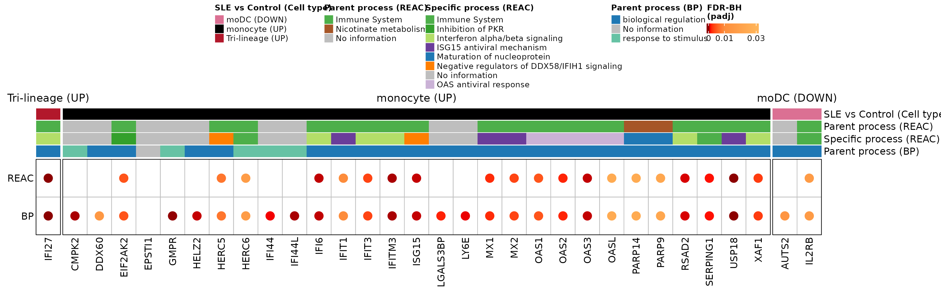

The monocyte ISGs are concentrated in the Reactome immune system, in specific antiviral processes: interferon alpha/beta signaling, the ISG15 antiviral mechanism, and the OAS antiviral response. This is the molecular footprint of interferon in lupus.

Challenge 3. Which monocyte genes take part in the Reactome term “Interferon alpha/beta signaling”?

Hint: filter go_results by query, source, and term_name, and look at the intersection column.

Show solution

go_results %>%
  filter(query == "SLE_UP_monocyte", source == "REAC",
         term_name == "Interferon alpha/beta signaling") %>%
  dplyr::select(term_name, intersection_size, term_size, p_value, intersection)
#>                         term_name intersection_size term_size      p_value
#> 1 Interferon alpha/beta signaling                16        76 1.032738e-25
#>                                                                               intersection
#> 1 EIF2AK2,IFI27,IFI6,IFIT1,IFIT3,IFITM3,ISG15,MX1,MX2,OAS1,OAS2,OAS3,OASL,RSAD2,USP18,XAF1

Challenge 4. In which databases is ABCA1 (up-regulated in tolDCs) annotated, and what is its specific process in Reactome?

Hint: use gene_source and process_info.

Show solution

gene_source %>% filter(gene == "ABCA1")
#> # A tibble: 7 × 2
#>   gene  source
#>   <chr> <chr> 
#> 1 ABCA1 BP    
#> 2 ABCA1 CC    
#> 3 ABCA1 MF    
#> 4 ABCA1 HP    
#> 5 ABCA1 KEGG  
#> 6 ABCA1 REAC  
#> 7 ABCA1 WP
process_info %>% filter(gene == "ABCA1")
#> # A tibble: 2 × 4
#>   source gene  specific_process                                   parent_process
#>   <chr>  <chr> <chr>                                              <chr>         
#> 1 GO:BP  ABCA1 positive regulation of high-density lipoprotein p… cellular resp…
#> 2 REAC   ABCA1 Defective ABCA1 causes TGD                         Transport of …

ABCA1 takes part in cholesterol transport: an example of the lipid metabolism alterations in the patients’ tolDCs.

7. Step 5: processes of all the DEGs (Supplementary Figure S4)

Figure 3D showed only the ISGs. Let us repeat the analysis with all the DEGs that have an annotation in Reactome or GO:BP, grouping them by their Reactome parent process:

s4_info <- gene_info %>%
  filter(gene %in% process_info$gene) %>%
  mutate(reac_parent   = factor(process_of("REAC", "parent_process", gene),
                                levels = names(reac_parent_color)),
         reac_specific = process_of("REAC", "specific_process", gene),
         bp_parent     = process_of("GO:BP", "parent_process", gene)) %>%
  arrange(reac_parent, gene)

nrow(s4_info)                   # DEGs with annotation in REAC or GO:BP
#> [1] 75
dplyr::count(s4_info, reac_parent)
#>                                     reac_parent  n
#> 1                                 Immune System 33
#> 2                Mitotic Metaphase and Anaphase  2
#> 3                          Metabolism of lipids  3
#> 4                  Transport of small molecules  2
#> 5 Respiratory Syncytial Virus Infection Pathway  1
#> 6                         Nicotinate metabolism  2
#> 7                                No information 32

As in Figure 3D, each cell holds the gene’s differential expression padj if it has an annotation in that database:

s4_padj <- sapply(c(REAC = "REAC", BP = "GO:BP"), function(src) {
  annotated <- s4_info$gene %in% process_info$gene[process_info$source == src]
  ifelse(annotated, s4_info$padj, NA)
})
rownames(s4_padj) <- s4_info$gene
head(s4_padj)
#>              REAC         BP
#> CARD11 0.04425396 0.04425396
#> CD28   0.02831443 0.02831443
#> CD40LG 0.01483254 0.01483254
#> CD96   0.01135195 0.01135195
#> CFI    0.02067849 0.02067849
#> DEFA1B 0.02095546 0.02095546

ht_s4 <- Heatmap(
  s4_padj, col = padj_color, na_col = "#f0f0f0",
  border = TRUE, rect_gp = gpar(col = "white", lwd = 2),
  cluster_rows = FALSE, cluster_columns = FALSE, row_names_side = "right",
  left_annotation = rowAnnotation(
    "Parent process (REAC)"   = as.character(s4_info$reac_parent),
    "Specific process (REAC)" = s4_info$reac_specific,
    "Parent process (BP)"     = s4_info$bp_parent,
    col = list("Parent process (REAC)"   = reac_parent_color,
               "Specific process (REAC)" = reac_specific_color,
               "Parent process (BP)"     = bp_parent_color)),
  right_annotation = rowAnnotation(
    "SLE vs Control\n(Cell type)" = s4_info$pattern,
    col = list("SLE vs Control\n(Cell type)" = pattern_color),
    annotation_legend_param = list("SLE vs Control\n(Cell type)" = list(nrow = 3))),
  row_split = droplevels(s4_info$reac_parent), row_title_rot = 0,
  heatmap_legend_param = list(title = "FDR-BH\n(padj)", at = c(0, 0.001, 0.01, 0.05)),
  width = unit(2, "cm"))

draw(ht_s4, merge_legends = TRUE)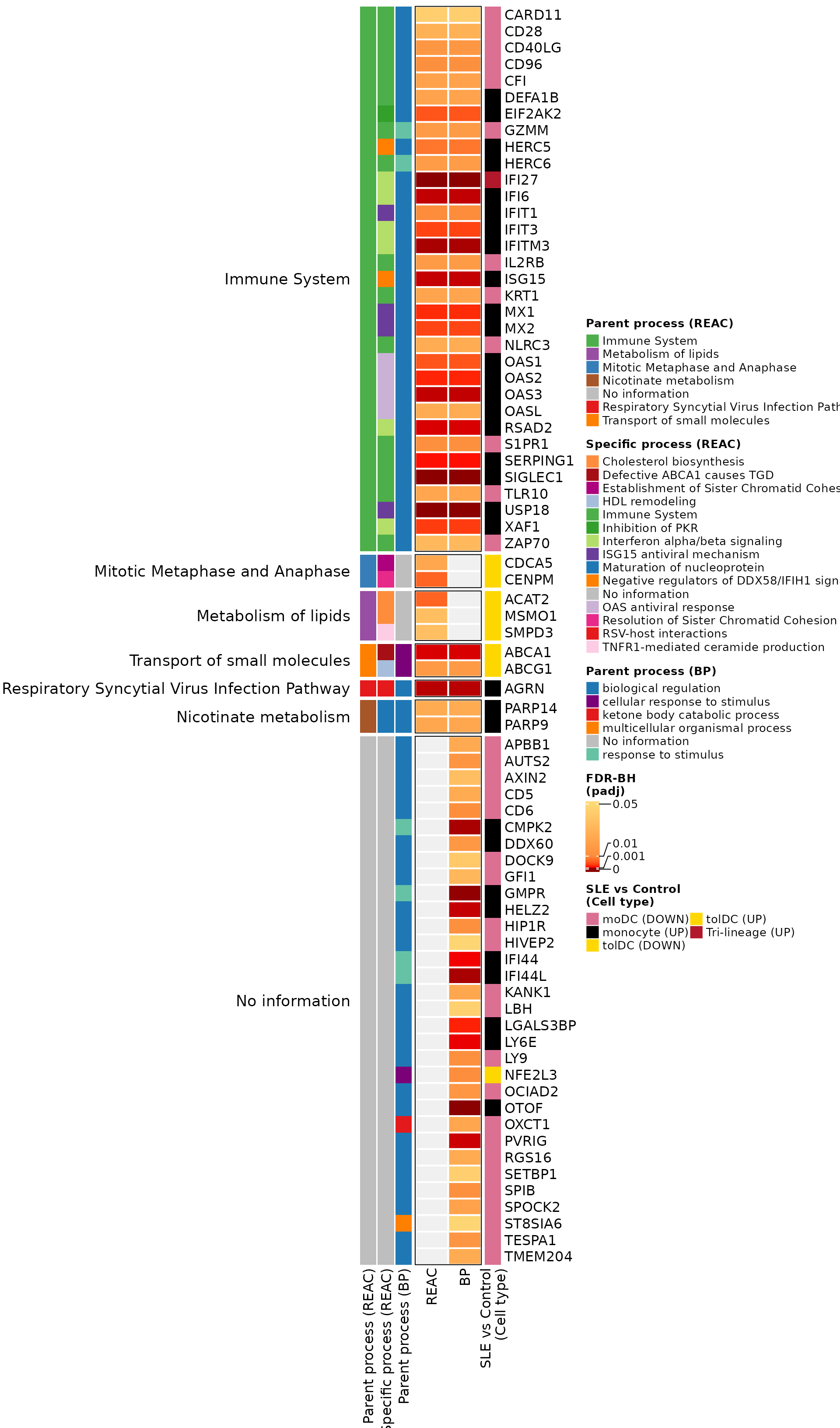

What do you observe?

The largest block is “Immune System”: it brings together the monocyte ISGs and also T-cell genes that go down in moDCs (CD28, CD40LG, ZAP70, CARD11).
The tolDC genes form their own groups: lipid metabolism (ACAT2, MSMO1, SMPD3) and transport of small molecules (ABCA1, ABCG1). This is the lipid alteration we saw in Challenge 1.
Many genes without information in Reactome do have annotation in GO:BP, mostly as “biological regulation”.

Supplementary Figure S4. Biological processes associated with the DEGs obtained when comparing SLE against Ctrl in each cell type. Processes were classified according to the parent and specific categories of Reactome (REAC) and the parent terms of Gene Ontology Biological Process (GO:BP). The REAC parent processes include the immune system, cell division (Mitotic Metaphase and Anaphase), lipid metabolism, and transport of small molecules. The color scale represents the differential expression padj (FDR-BH) of each gene, with a maximum threshold of padj < 0.05; gray cells indicate that the gene has no annotation in that database. DEGs: differentially expressed genes.

The original supplementary figure can be found in the supplementary material of the article.

8. To finish: Figure 3 of the article

We capture the heatmaps as graphical objects (as in the previous lesson) and join them with the dot plots:

grab <- function(ht, ...) {
  grid::grid.grabExpr(draw(ht, merge_legends = TRUE, heatmap_legend_side = "top",
                           annotation_legend_side = "top", ...), wrap.grobs = TRUE)
}

figure_3 <- plot_grid(
  grab(ht_fig3a, ht_gap = unit(5, "mm")),
  p_sle,
  p_isg,
  grab(ht_fig3d),
  labels = c("A", "B", "C", "D"), label_size = 20, ncol = 1,
  rel_heights = c(3.2, 0.9, 0.9, 1)
)
figure_3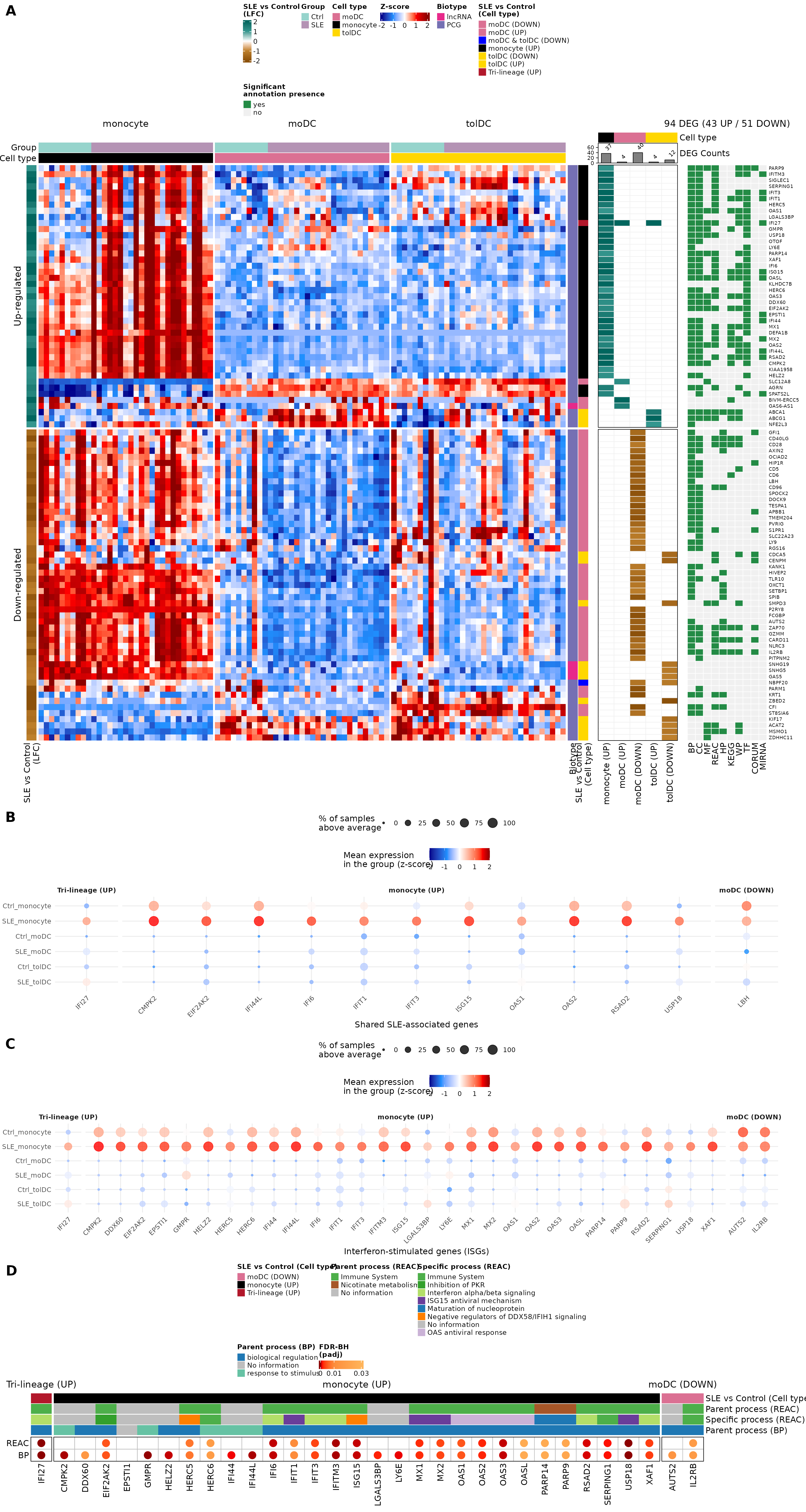

Figure 3. The functional enrichment analysis reveals cell type-specific perturbations and a shared lupus signature. (A) Integrated view of the DEGs and their functional enrichment. Left: heatmap of the 94 DEGs (43 up-regulated and 51 down-regulated) between SLE and Ctrl in the three cell types, selected with |LFC| ≥ 1 and padj < 0.05; the color scale corresponds to z-scores. Center: LFC of SLE versus Ctrl in each DEG list, with a barplot of the number of DEGs per list. Right: presence of significant functional terms (g:Profiler; hypergeometric test) in GO (BP, CC, MF), REAC, HP, KEGG, WP, TF, CORUM, and miRNA. (B, C) Mean expression (z-score) by group and cell type (rows) of (B) the SLE-associated DEGs and (C) the differentially expressed ISGs; the dot size indicates the percentage of samples above each gene’s average. Genes are grouped by their pattern: “Tri-lineage (UP)” goes up in all three cell types, “monocyte (UP)” goes up in monocytes, and “moDC (DOWN)” goes down in moDCs. (D) Biological processes associated with the differentially expressed ISGs, according to the Reactome (REAC) parent and specific terms and the GO:BP parent terms. Circles indicate that the gene has an annotation in that database; their color represents the gene’s differential expression padj (FDR-BH).

The original figure can be found in the article.

To save it in high resolution:

ggsave("Figure_3.png", figure_3, width = 16, height = 30, dpi = 300)

ISG expression clearly separates patients from controls. A natural question is whether, among patients, ISGs are higher when the disease is more active. To answer it we correlate the z-score of each of the 32 ISGs with the SLEDAI score using Spearman correlation, which compares ranks and does not assume a linear relationship or normal data.

First we join the ISG z-scores with the SLEDAI of each patient sample. Each patient contributes three samples (monocyte, moDC and tolDC); the patient identifier is the part of sample_ID before the underscore:

sle_info <- metadata_cleaned %>%
  filter(Group == "SLE") %>%
  mutate(sample_ID = as.character(sample_ID),
         patient   = sub("_.*", "", sample_ID),                # QR011_0 → QR011
         SLEDAI    = as.numeric(as.character(Sledai_score))) %>%
  dplyr::select(sample_ID, patient, Cell_type, SLEDAI)

isg_long <- zscore_mat[isg_deg, ] %>%
  as.data.frame() %>%
  rownames_to_column("gene") %>%
  pivot_longer(-gene, names_to = "sample_ID", values_to = "zscore") %>%
  inner_join(sle_info, by = "sample_ID")

# disease activity, as in Table 1 (lesson 1):
# 1 = active (SLEDAI ≥ 6), 0 = no or low activity (0-5)
sle_activity <- volunteer_info %>% filter(Group == "SLE")
dplyr::count(sle_activity, SLEDAI)
#>   SLEDAI  n
#> 1      0 13
#> 2      1 10

Only 10 of the 23 patients (43.5%) have active disease; the rest have no or low activity. With few active patients, the power to detect a correlation is limited.

We save the test in a function. Since we test 32 genes at once, we correct the p-values for multiple testing with FDR, just as DESeq2 does with padj:

spearman <- function(df) {
  test <- cor.test(df$zscore, df$SLEDAI, method = "spearman", exact = FALSE)
  tibble(rho = unname(test$estimate), p_value = test$p.value)
}

9.1 Without separating by cell type

To avoid counting the same patient three times, we average the z-score of the patient’s three cell types before correlating:

cor_overall <- isg_long %>%
  group_by(gene, patient, SLEDAI) %>%
  summarise(zscore = mean(zscore), .groups = "drop") %>%
  group_by(gene) %>%
  group_modify(~ spearman(.x)) %>%
  ungroup() %>%
  mutate(FDR = p.adjust(p_value, method = "fdr")) %>%
  arrange(p_value)

knitr::kable(cor_overall, digits = 3, col.names = c("Gene", "rho", "p", "FDR"))

Gene	rho	p	FDR
OAS2	0.312	0.148	0.903
MX1	0.268	0.216	0.903
IFIT3	0.254	0.242	0.903
RSAD2	0.244	0.262	0.903
CMPK2	0.241	0.267	0.903
HERC6	0.237	0.275	0.903
DDX60	0.231	0.289	0.903
PARP9	0.231	0.289	0.903
IFI6	0.214	0.327	0.903
OASL	0.201	0.358	0.903
IL2RB	-0.200	0.360	0.903
LGALS3BP	0.179	0.414	0.903
EIF2AK2	0.164	0.454	0.903
XAF1	0.163	0.458	0.903
USP18	0.152	0.490	0.903
OAS3	0.149	0.497	0.903
LY6E	0.147	0.504	0.903
IFI44	0.136	0.537	0.903
IFI27	0.127	0.564	0.903
GMPR	0.112	0.612	0.903
EPSTI1	0.095	0.665	0.903
MX2	0.088	0.690	0.903
IFIT1	0.087	0.692	0.903
AUTS2	-0.081	0.714	0.903
IFI44L	0.074	0.736	0.903
PARP14	0.070	0.751	0.903
ISG15	-0.067	0.762	0.903
OAS1	0.052	0.812	0.928
IFITM3	-0.030	0.890	0.958
HELZ2	-0.022	0.921	0.958
SERPING1	0.020	0.928	0.958
HERC5	-0.003	0.987	0.987

Supplementary Table (a). Spearman correlation between the normalized expression (z-score) of the 32 differentially expressed ISGs and disease activity (SLEDAI) in 23 SLE patients, without separating by cell type (mean z-score of each patient’s monocytes, moDCs and tolDCs). The number of genes with p < 0.05 is 0, and none is significant after correction for multiple testing (minimum FDR = 0.90). rho, Spearman correlation coefficient; FDR, false discovery rate (Benjamini-Hochberg); ISG, interferon-stimulated genes; SLEDAI, SLE Disease Activity Index.

9.2 By cell type

Now we repeat the test within each cell type (23 samples per type) and correct by FDR within each one:

cor_celltype <- isg_long %>%
  group_by(Cell_type, gene) %>%
  group_modify(~ spearman(.x)) %>%
  group_by(Cell_type) %>%
  mutate(FDR = p.adjust(p_value, method = "fdr")) %>%
  ungroup() %>%
  mutate(Cell_type = factor(Cell_type, levels = c("monocyte", "moDC", "tolDC")))

cor_celltype %>%
  pivot_wider(id_cols = gene, names_from = Cell_type, values_from = c(rho, p_value, FDR),
              names_vary = "slowest", names_sort = TRUE) %>%
  arrange(gene) %>%
  knitr::kable(digits = 3,
               col.names = c("Gene", paste(c("rho", "p", "FDR"), rep(levels(cor_celltype$Cell_type), each = 3))))

Gene	rho monocyte	p monocyte	FDR monocyte	rho moDC	p moDC	FDR moDC	rho tolDC	p tolDC	FDR tolDC
AUTS2	0.010	0.962	0.962	-0.276	0.203	0.726	-0.149	0.498	0.948
CMPK2	0.191	0.382	0.582	0.141	0.522	0.726	0.258	0.234	0.948
DDX60	0.165	0.453	0.582	0.175	0.424	0.726	0.174	0.428	0.948
EIF2AK2	0.167	0.447	0.582	0.256	0.239	0.726	0.054	0.805	0.968
EPSTI1	0.168	0.445	0.582	0.113	0.608	0.775	0.029	0.894	0.968
GMPR	0.280	0.196	0.582	-0.262	0.227	0.726	0.175	0.426	0.948
HELZ2	0.162	0.460	0.582	-0.238	0.273	0.726	-0.127	0.563	0.948
HERC5	0.155	0.480	0.582	0.077	0.726	0.860	-0.229	0.292	0.948
HERC6	0.185	0.399	0.582	0.415	0.049	0.726	0.139	0.528	0.948
IFI27	0.204	0.352	0.582	0.213	0.328	0.726	0.021	0.923	0.968
IFI44	0.173	0.430	0.582	0.161	0.464	0.726	0.099	0.652	0.968
IFI44L	0.151	0.491	0.582	0.109	0.620	0.775	-0.009	0.968	0.968
IFI6	0.262	0.227	0.582	0.213	0.330	0.726	0.246	0.257	0.948
IFIT1	0.154	0.482	0.582	0.036	0.871	0.912	-0.011	0.959	0.968
IFIT3	0.174	0.428	0.582	0.385	0.070	0.726	0.091	0.679	0.968
IFITM3	0.248	0.254	0.582	-0.219	0.316	0.726	-0.245	0.260	0.948
IL2RB	-0.169	0.440	0.582	-0.067	0.760	0.869	-0.132	0.548	0.948
ISG15	0.116	0.597	0.628	-0.266	0.219	0.726	-0.173	0.430	0.948
LGALS3BP	0.212	0.333	0.582	0.180	0.412	0.726	0.016	0.941	0.968
LY6E	0.251	0.247	0.582	0.032	0.883	0.912	0.226	0.301	0.948
MX1	0.184	0.402	0.582	0.243	0.263	0.726	0.290	0.180	0.948
MX2	0.166	0.449	0.582	0.022	0.919	0.919	-0.068	0.757	0.968
OAS1	0.196	0.371	0.582	0.052	0.812	0.896	-0.200	0.361	0.948
OAS2	0.244	0.261	0.582	0.374	0.079	0.726	0.238	0.274	0.948
OAS3	0.174	0.427	0.582	0.142	0.519	0.726	-0.165	0.451	0.948
OASL	0.113	0.608	0.628	0.178	0.418	0.726	0.032	0.885	0.968
PARP14	0.136	0.537	0.614	0.175	0.424	0.726	-0.009	0.966	0.968
PARP9	0.206	0.347	0.582	0.141	0.522	0.726	-0.110	0.618	0.968
RSAD2	0.207	0.343	0.582	0.171	0.436	0.726	0.197	0.367	0.948
SERPING1	0.239	0.272	0.582	-0.106	0.629	0.775	-0.341	0.111	0.948
USP18	0.169	0.440	0.582	0.242	0.266	0.726	0.086	0.697	0.968
XAF1	0.128	0.561	0.619	-0.196	0.371	0.726	0.200	0.360	0.948

Supplementary Table (b). Spearman correlation between the normalized expression (z-score) of the 32 differentially expressed ISGs and disease activity (SLEDAI) in each cell type (monocytes, moDCs and tolDCs; 23 SLE patients per cell type). P-values were FDR-corrected within each cell type. 1 of the 96 tests has p < 0.05 and none is significant after correction (minimum FDR = 0.58). rho, Spearman correlation coefficient; FDR, false discovery rate (Benjamini-Hochberg); ISG, interferon-stimulated genes; moDC, monocyte-derived dendritic cells; tolDC, tolerogenic dendritic cells; SLEDAI, SLE Disease Activity Index.

The original table (Supplementary Table 8) can be found in the article’s supplementary material.

What do you notice?

Some genes show nominal associations (p < 0.05) in one cell type, but no correlation survives multiple-testing correction.
ISGs separate patients from controls but, in this cohort, no individual ISG tracks disease activity.
Possible reasons: immunomodulatory treatments, the in vitro differentiation dampening the inflammatory signals the cells carried from the patient, and the fact that most patients have low activity.

What can and cannot be concluded?

We can say that, in this cohort, we did not detect a significant association between ISG expression and SLEDAI, either without separating by cell type or within each cell type.
We cannot conclude that ISGs are unrelated to lupus activity. A non-significant result is absence of evidence, not evidence of absence: with 23 patients, a correlation needs |rho| above ~0.41 to reach p < 0.05, and even more after FDR correction. Moderate correlations would go unnoticed.
Nor can we treat as a finding a nominal association (uncorrected p < 0.05): with 96 tests, we would expect ~5 p-values < 0.05 by chance alone.
It is consistent with Challenge 3 of lesson 2: in the PCA, samples do not separate by disease activity either.
To answer it would require a larger cohort, with more active patients, and measuring ISGs directly in uncultured cells.

10. Summary

Step	Key function	What for?
DEG lists	`filter()`, `split()`	Separate genes by cell type and direction
Enrichment	`gprofiler2::gost()`	Find overrepresented functions
Reproducibility	`set_base_url()`	Pin the database version
Explore terms	`slice_min(p_value)`	See the most significant processes
Genes per term	`separate_rows()`	Go from “term → genes” to “gene → terms”
Reference lists	`intersect()`	Find SLE genes and ISGs among the DEGs
ISG enrichment	`phyper()`, `fisher.test()`	Test whether there are more ISGs than expected by chance
Integrate	heatmaps with `+`	See expression, LFC, and annotations together
Correlation	`cor.test(method = "spearman")`, `p.adjust()`	Relate expression to disease activity

Common beginner mistakes

Interpreting enrichment as causation: it indicates functional association, not mechanism.
Not reporting the database version: results change over time.
Using very small lists: with 4 genes (moDC UP) there is almost no power; the terms that come out may depend on a single gene.
Mixing up- and down-regulated genes in a single list: it can dilute opposing signals.
Ignoring term size: a term with 5,000 genes is very general; one with 20 is more informative.

11. Next steps

So far we have compared patients against controls within each cell type. The lesson Differentiation of monocytes into dendritic cells poses a different question: what changes when a monocyte differentiates into a dendritic cell?, and does it happen in the same way in patients and in controls?

To continue, click the Next lesson: Monocyte differentiation button at the bottom of this page.

↑ Back to top

Session information

sessionInfo()
#> R version 4.6.2 (2026-10-29)
#> Platform: x86_64-pc-linux-gnu
#> Running under: Ubuntu 24.04.5 LTS
#> 
#> Matrix products: default
#> BLAS:   /usr/lib/x86_64-linux-gnu/openblas-pthread/libblas.so.3 
#> LAPACK: /usr/lib/x86_64-linux-gnu/openblas-pthread/libopenblasp-r0.3.26.so;  LAPACK version 3.12.0
#> 
#> locale:
#>  [1] LC_CTYPE=C.UTF-8       LC_NUMERIC=C           LC_TIME=C.UTF-8       
#>  [4] LC_COLLATE=C.UTF-8     LC_MONETARY=C.UTF-8    LC_MESSAGES=C.UTF-8   
#>  [7] LC_PAPER=C.UTF-8       LC_NAME=C              LC_ADDRESS=C          
#> [10] LC_TELEPHONE=C         LC_MEASUREMENT=C.UTF-8 LC_IDENTIFICATION=C   
#> 
#> time zone: UTC
#> tzcode source: system (glibc)
#> 
#> attached base packages:
#> [1] grid      stats     graphics  grDevices utils     datasets  methods  
#> [8] base     
#> 
#> other attached packages:
#>  [1] cowplot_1.2.0              circlize_0.4.18           
#>  [3] ComplexHeatmap_2.28.0      lubridate_1.9.5           
#>  [5] forcats_1.0.1              stringr_1.6.0             
#>  [7] dplyr_1.2.1                purrr_1.2.2               
#>  [9] readr_2.2.0                tidyr_1.3.2               
#> [11] tibble_3.3.1               ggplot2_4.0.3             
#> [13] tidyverse_2.0.0            GeneExprLupusMx_0.1.0.9000
#> 
#> loaded via a namespace (and not attached):
#>  [1] shape_1.4.6.1       gtable_0.3.6        rjson_0.2.23       
#>  [4] xfun_0.62           bslib_0.12.0        GlobalOptions_0.1.4
#>  [7] tzdb_0.5.0          vctrs_0.7.3         tools_4.6.2        
#> [10] generics_0.1.4      stats4_4.6.2        parallel_4.6.2     
#> [13] cluster_2.1.8.3     pkgconfig_2.0.3     RColorBrewer_1.1-3 
#> [16] S7_0.2.2            desc_1.4.3          S4Vectors_0.50.3   
#> [19] lifecycle_1.0.5     compiler_4.6.2      farver_2.1.2       
#> [22] textshaping_1.0.5   codetools_0.2-20    clue_0.3-68        
#> [25] htmltools_0.5.9     sass_0.4.10         yaml_2.3.12        
#> [28] pillar_1.11.1       pkgdown_2.2.1       crayon_1.5.3       
#> [31] jquerylib_0.1.4     cachem_1.1.0        iterators_1.0.14   
#> [34] foreach_1.5.2       ggh4x_0.3.1         tidyselect_1.2.1   
#> [37] digest_0.6.39       stringi_1.8.9       labeling_0.4.3     
#> [40] fastmap_1.2.0       colorspace_2.1-4    cli_3.6.6          
#> [43] magrittr_2.0.5      utf8_1.2.6          withr_3.0.3        
#> [46] scales_1.4.0        timechange_0.4.0    rmarkdown_2.32     
#> [49] matrixStats_1.5.0   otel_0.2.0          ragg_1.5.2         
#> [52] png_0.1-9           GetoptLong_1.1.1    hms_1.1.4          
#> [55] evaluate_1.0.5      knitr_1.52          IRanges_2.46.0     
#> [58] doParallel_1.0.17   rlang_1.3.0         glue_1.8.1         
#> [61] BiocGenerics_0.58.1 jsonlite_2.0.0      R6_2.6.1           
#> [64] systemfonts_1.3.2   fs_2.1.0

Functional enrichment analysis with g:Profiler

2026-10-31

Welcome

Lesson map

Glossary

1. Setup

Starting point: the DEGs from the previous lesson

2. What is an enrichment analysis?

3. Step 1: enrichment with g:Profiler

3.1 The most significant terms

4. Step 2: overview of the 94 DEGs (Figure 3A)

4.1 Expression heatmap

4.2 LFC heatmap by list

4.3 Annotation heatmap

4.4 All three together

5. Step 3: lupus-associated genes and ISGs (Figures 3B and 3C)

5.1 Are there more ISGs than expected by chance?

6. Step 4: which processes do the ISGs take part in? (Figure 3D)

7. Step 5: processes of all the DEGs (Supplementary Figure S4)

8. To finish: Figure 3 of the article

9.1 Without separating by cell type

9.2 By cell type

10. Summary

Common beginner mistakes

11. Next steps

Session information

Lesson 4: Biological functions of differentially expressed genes

Functional enrichment analysis with g:Profiler

2026-10-31

Welcome

Lesson map

Glossary

1. Setup

Starting point: the DEGs from the previous lesson

2. What is an enrichment analysis?

3. Step 1: enrichment with g:Profiler

3.1 The most significant terms

4. Step 2: overview of the 94 DEGs (Figure 3A)

4.1 Expression heatmap

4.2 LFC heatmap by list

4.3 Annotation heatmap

4.4 All three together

5. Step 3: lupus-associated genes and ISGs (Figures 3B and 3C)

5.1 Are there more ISGs than expected by chance?

6. Step 4: which processes do the ISGs take part in? (Figure 3D)

7. Step 5: processes of all the DEGs (Supplementary Figure S4)

8. To finish: Figure 3 of the article

9. Going further: are ISGs related to disease activity?

9.1 Without separating by cell type

9.2 By cell type

10. Summary

Common beginner mistakes

11. Next steps

Session information