Lesson 3: Differentially expressed genes between patients and controls

Welcome

In the previous lessons you met the participants and explored gene expression: you saw that cell type dominates the variation and that some patients have an interferon signature. Now we will ask the central question of the study using statistics: which genes change their expression in lupus, within each cell type?

What you need to know beforehand: having completed the lesson From RNA-seq counts to data exploration (normalization, VST, z-scores, and PCA).

By the end you will be able to:

Validate the identity of the cell types with biomarker genes.
Run a differential expression analysis with DESeq2 and understand each column of its results.
Define differentially expressed genes (DEGs) with thresholds on the log2 fold change and the adjusted p-value.
Build and interpret volcano plots.
Reproduce Figure 2 of the article.

Estimated time: 1.5 hours.

Lesson map

flowchart LR
  A["Package data
counts + metadata"] --> B["1. Biomarkers:
are these the right cells?"]
  A --> C["2. Global heatmap
by cell type"]
  A --> D["3. DESeq2:
SLE vs Ctrl by cell type"]
  D --> E["4. DEGs:
|LFC| ≥ 1 and padj < 0.05"]
  E --> F["5. Volcano plots"]
  B --> G["Figure 2"]
  C --> G
  F --> G

Glossary

These are the terms we will use. Come back here whenever you need to.

Biomarker: a gene whose expression characterizes a cell type.
Differential expression: difference in the expression of a gene between two conditions (here, SLE versus Ctrl).
DEG (differentially expressed gene): a gene that is differentially expressed according to the thresholds we choose.
Fold change: how many times the expression changes. A fold change of 2 means double.
log2 fold change (LFC): the fold change on a log2 scale. LFC = 1 is double; LFC = −1, half; LFC = 0, no change.
Wald test: test used by DESeq2 to assess whether the LFC is different from zero.
p-value: probability of observing data as extreme as ours if the null hypothesis were true (here, if there were actually no difference).
Multiple comparisons: when testing thousands of genes, some will come out significant by chance.
FDR (false discovery rate): expected proportion of false positives among the genes we declare significant.
Benjamini–Hochberg (BH): method that corrects p-values to control the FDR.
padj: p-value adjusted by BH. This is the one used to decide.
Independent filtering: DESeq2 does not compute padj for genes with very few reads, because they lack statistical power; they are left as NA.
Volcano plot: plot of the LFC (x axis) against significance (y axis) for all genes.

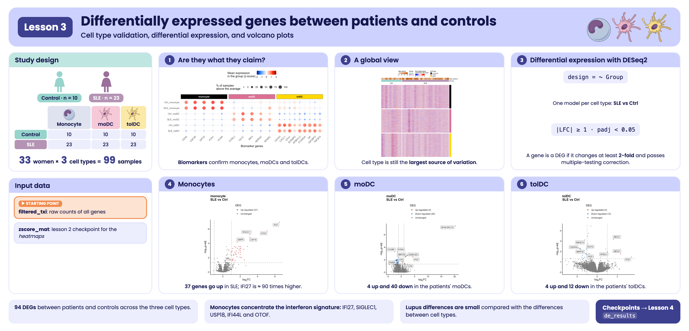
Visual summary of lesson 3.

1. Setup

library(GeneExprLupusMx) # package data and heatmap functions
library(DESeq2)          # differential expression
library(tidyverse)       # table manipulation and plots
library(ComplexHeatmap)  # heatmaps
library(circlize)        # color scales for ComplexHeatmap
library(ggrepel)         # non-overlapping labels
library(cowplot)         # combine plots into a panel

# Large package objects: downloaded only the first time (see ?download_data)
filtered_txi <- download_data("filtered_txi")
zscore_mat   <- download_data("zscore_mat")

Colors and thresholds we will use throughout the lesson:

cell_color  <- c(monocyte = "black", moDC = "palevioletred", tolDC = "gold1")
group_color <- c(Ctrl = "#96d4ccff", SLE = "#b493b4ff")

lfc_threshold  <- 1    # minimum |log2 fold change|
padj_threshold <- 0.05 # maximum adjusted p-value

Starting point

This lesson uses the package data: the counts (filtered_txi), the metadata (metadata_cleaned), the volunteer information (volunteer_info), and the zscore_mat checkpoint from the previous lesson.

For the differential expression analysis we start from the raw counts of all genes. We create a DESeqDataSet object with the design ~ Group (SLE versus Ctrl), which we will later split by cell type:

metadata_cleaned$Group <- relevel(metadata_cleaned$Group, ref = "Ctrl")

full_dds <- DESeqDataSetFromTximport(txi     = filtered_txi,
                                     colData = metadata_cleaned,
                                     design  = ~ Group)
full_dds
#> class: DESeqDataSet 
#> dim: 21718 99 
#> metadata(1): version
#> assays(2): counts avgTxLength
#> rownames(21718): A1BG A1BG-AS1 ... ZZEF1 ZZZ3
#> rowData names(0):
#> colnames(99): QR011_0 QR011_1 ... QR108_1 QR108_3
#> colData names(14): sample_ID Group ... SLEDAI_Md SLEDAI_category

Why don’t we use the dds checkpoint? In the previous lesson we filtered lowly expressed genes for visualization. For differential expression this is not needed: DESeq2 applies its own independent filtering and leaves padj = NA for genes without information. Starting from all the counts lets DESeq2 decide which genes have enough information to be tested.

2. Step 1: are the cells what they claim to be?

Before comparing patients against controls, let us check that each sample is of the cell type it claims to be. For this we use biomarkers: genes known to be expressed in one cell type and not in the others.

markers <- list(
  monocyte = c("CD36", "CSF3R", "DPYD", "FCN1", "VCAN"),
  moDC     = c("CD1C", "IRF4", "NDRG2", "CCRL2", "SPARC"), # as in the published Figure 2B
  tolDC    = c("IGF2BP3", "CD163", "FCGR2A", "DTX1", "GK", "EPB41L3", "TNFSF9", "CXCL1", "EFEMP2")
)
marker_genes <- unlist(markers)
all(marker_genes %in% rownames(zscore_mat)) # are they all in the data?
#> [1] TRUE

For each combination of group and cell type we calculate two numbers per gene, based on the z-scores:

Mean expression (z-score): positive if the gene is above its average in that group.
Percentage of samples above the average (z-score > 0): how consistent that expression is across the samples in the group.

marker_df <- as.data.frame(zscore_mat[marker_genes, ]) %>%
  rownames_to_column("gene") %>%
  pivot_longer(-gene, names_to = "sample_ID", values_to = "expression") %>%
  left_join(dplyr::select(metadata_cleaned, sample_ID, Group, Cell_type), by = "sample_ID") %>%
  group_by(Group, Cell_type, gene) %>%
  summarise(mean_expression = mean(expression),
            pct_expressed   = 100 * mean(expression > 0),
            .groups = "drop") %>%
  mutate(condition    = paste(Group, Cell_type, sep = "_"),
         marker_group = factor(case_when(gene %in% markers$monocyte ~ "monocyte",
                                         gene %in% markers$moDC     ~ "moDC",
                                         gene %in% markers$tolDC    ~ "tolDC"),
                               levels = names(markers)))
head(marker_df)
#> # A tibble: 6 × 7
#>   Group Cell_type gene  mean_expression pct_expressed condition marker_group
#>   <fct> <fct>     <chr>           <dbl>         <dbl> <chr>     <fct>       
#> 1 Ctrl  moDC      CCRL2           0.451            60 Ctrl_moDC moDC        
#> 2 Ctrl  moDC      CD163          -0.829            20 Ctrl_moDC tolDC       
#> 3 Ctrl  moDC      CD1C            1.18             90 Ctrl_moDC moDC        
#> 4 Ctrl  moDC      CD36           -0.264            20 Ctrl_moDC monocyte    
#> 5 Ctrl  moDC      CSF3R          -0.893             0 Ctrl_moDC monocyte    
#> 6 Ctrl  moDC      CXCL1          -0.721            10 Ctrl_moDC tolDC

We plot it as a dot plot: the color is the mean expression and the size is the percentage of samples.

# minimum and maximum mean expression, for the color scale
min_val <- min(marker_df$mean_expression, na.rm = TRUE)
max_val <- max(marker_df$mean_expression, na.rm = TRUE)

p_markers <- marker_df %>%
  mutate(condition = factor(condition, levels = c("SLE_tolDC", "Ctrl_tolDC", "SLE_moDC",
                                                  "Ctrl_moDC", "SLE_monocyte", "Ctrl_monocyte"))) %>%
  ggplot(aes(x = gene, y = condition, color = mean_expression, size = pct_expressed)) +
  geom_point(alpha = 0.8) +
  scale_color_gradientn(
    colors = c("darkblue", "dodgerblue", "white", "red", "darkred"),
    values = scales::rescale(c(-2, min_val, 0, max_val, 2)),
    limits = c(-2, 2),
    oob = scales::squish # values outside [-2, 2] take the color of the end
  ) +
  ggh4x::facet_wrap2(
    ~ marker_group, scales = "free_x", nrow = 1,
    strip = ggh4x::strip_themed(
      background_x = lapply(cell_color, function(col) element_rect(fill = col)),
      text_x = list(element_text(color = "white", face = "bold"),
                    element_text(color = "white", face = "bold"),
                    element_text(color = "black", face = "bold")))) +
  labs(x = "Biomarker genes", y = NULL,
       color = "Mean expression\nin the group (z-score)",
       size = "% of samples\nabove the average") +
  theme_minimal(base_size = 13) +
  theme(legend.position = "top", legend.box = "vertical",
        axis.text.x = element_text(angle = 45, hjust = 1))
p_markers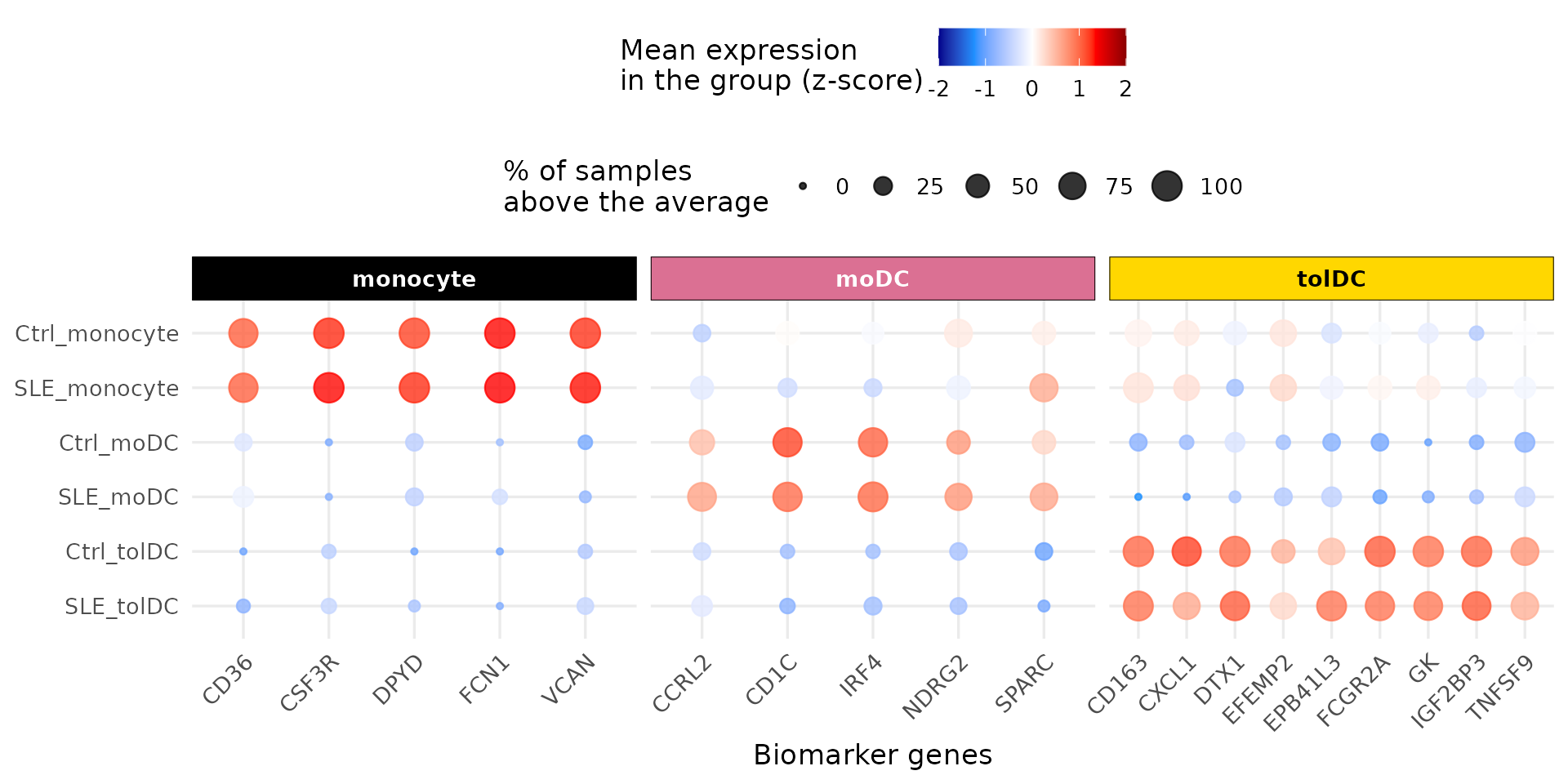

What do you observe? Each group of biomarkers is red (high expression) exactly in its own cell type, in both controls and patients, and blue in the others. The identity of the samples is correct: we can trust the comparisons we will make.

3. Step 2: a global view with a heatmap

Before the statistics, let us look at all the genes at once. We will calculate the z-scores within each cell type (not across all samples), so that the color shows how each sample compares with the others of its own cell type.

The package function get_heatmap_mat() applies the VST transformation, removes genes with no variation, and calculates the z-scores:

cell_types <- c("monocyte", "moDC", "tolDC")

heatmap_mats <- lapply(cell_types, function(cell) {
  mat <- get_heatmap_mat(full_dds[, full_dds$Cell_type == cell])
  colnames(mat) <- sub("_.*", "", colnames(mat)) # QR011_0 -> QR011
  mat
})
names(heatmap_mats) <- cell_types
sapply(heatmap_mats, nrow) # genes with variation in each cell type
#> monocyte     moDC    tolDC 
#>    17142    16986    18045

We rename the columns with the volunteer identifier (QR011_0 → QR011): this way, in the three heatmaps, each column is the same person. We keep the genes present in all three and order the volunteers by group and disease activity:

common_genes <- Reduce(intersect, lapply(heatmap_mats, rownames))
length(common_genes)
#> [1] 16283

sample_info <- volunteer_info %>%
  arrange(Group, SLEDAI)

heatmap_mats <- lapply(heatmap_mats, function(mat) mat[common_genes, sample_info$Volunteer_ID])

Now we build one heatmap per cell type with the package’s create_heatmap() and stack them. At the top we add two annotations: the age and the group of each volunteer.

top_annotation <- HeatmapAnnotation(
  "Age (years)" = sample_info$Age_years,
  Group         = sample_info$Group,
  col = list("Age (years)" = colorRamp2(range(sample_info$Age_years), c("#e6d1be", "#bd5a00")),
             Group         = group_color),
  annotation_legend_param = list("Age (years)" = list(direction = "horizontal"))
)

heatmap_list <- create_heatmap(heatmap_mats$monocyte, cell_color[["monocyte"]], sample_info$Group) %v%
  create_heatmap(heatmap_mats$moDC,  cell_color[["moDC"]],  sample_info$Group) %v%
  create_heatmap(heatmap_mats$tolDC, cell_color[["tolDC"]], sample_info$Group)

cell_legend <- Legend(labels = cell_types, title = "Cell type",
                      legend_gp = grid::gpar(fill = cell_color))

ht_opt$message <- FALSE
draw(top_annotation %v% heatmap_list,
     merge_legends = TRUE, annotation_legend_list = list(cell_legend),
     annotation_legend_side = "top", heatmap_legend_side = "top")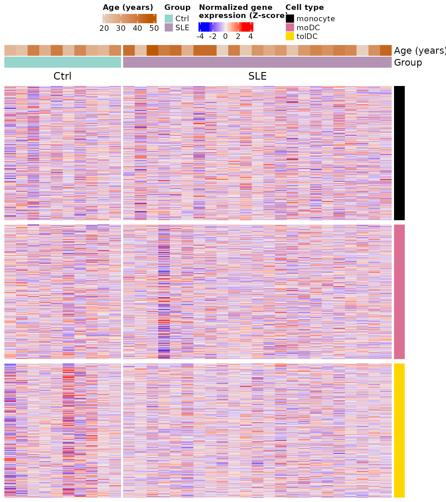

Each block is a cell type (color bar on the right), each row a gene, and each column a volunteer. No obvious pattern separates patients from controls: the differences, if they exist, are in relatively few genes and cannot be seen at a glance among more than 16,000. To find them we need statistics.

4. Step 3: differential expression with DESeq2

4.1 The question

For each gene, in each cell type, we ask: is its expression different in patients than in controls? We do the analysis separately for each cell type, because we already saw (in the PCA of the previous lesson) that cell type is the largest source of variation: mixing them would mask the differences due to lupus.

4.2 Step by step with monocytes

We select the 33 monocyte samples:

dds_mo <- full_dds[, full_dds$Cell_type == "monocyte"]
dds_mo$Cell_type <- droplevels(dds_mo$Cell_type) # remove levels that no longer exist
design(dds_mo) # ~ Group
#> ~Group
table(dds_mo$Group)
#> 
#> Ctrl  SLE 
#>   10   23

DESeq() does the whole analysis in a single function, in three steps:

Normalization: estimates the size factors (as in the previous lesson).
Dispersion: estimates how much each gene varies between replicates of the same group.
Model and test: fits a negative binomial model and uses the Wald test to assess whether the LFC between groups is different from zero.

dds_mo <- DESeq(dds_mo, quiet = TRUE)
resultsNames(dds_mo) # available comparisons
#> [1] "Intercept"         "Group_SLE_vs_Ctrl"

We extract the Group_SLE_vs_Ctrl comparison (SLE against the reference, Ctrl):

res_mo <- results(dds_mo, name = "Group_SLE_vs_Ctrl")
head(res_mo[order(res_mo$padj), ])
#> log2 fold change (MLE): Group SLE vs Ctrl 
#> Wald test p-value: Group SLE vs Ctrl 
#> DataFrame with 6 rows and 6 columns
#>          baseMean log2FoldChange     lfcSE      stat      pvalue        padj
#>         <numeric>      <numeric> <numeric> <numeric>   <numeric>   <numeric>
#> IFI27     745.809        6.50566  0.965817   6.73591 1.62908e-11 1.13758e-07
#> OTOF      725.570        5.08949  0.819047   6.21392 5.16796e-10 1.80439e-06
#> SIGLEC1  8360.445        3.11093  0.521640   5.96375 2.46508e-09 5.73787e-06
#> USP18     758.460        3.12316  0.541137   5.77148 7.85805e-09 1.37182e-05
#> GMPR      403.561        1.64509  0.301470   5.45691 4.84499e-08 6.76651e-05
#> IFI44L   6547.050        2.82422  0.550876   5.12678 2.94735e-07 2.72542e-04

What does each column mean?

Column	Meaning
`baseMean`	Mean normalized expression of the gene across all samples
`log2FoldChange`	LFC of SLE against Ctrl: positive = higher in patients; negative = lower
`lfcSE`	Standard error of the LFC (uncertainty of the estimate)
`stat`	Wald test statistic (LFC / lfcSE)
`pvalue`	p-value of the Wald test
`padj`	p-value adjusted by Benjamini–Hochberg (the one we use to decide)

IFI27 tops the list: its LFC of 6.5 means that in the patients’ monocytes it is expressed about 2^6.5 ≈ 90 times more than in controls. It is one of the interferon signature genes you saw in the previous lesson.

summary(res_mo, alpha = padj_threshold)
#> 
#> out of 17139 with nonzero total read count
#> adjusted p-value < 0.05
#> LFC > 0 (up)       : 76, 0.44%
#> LFC < 0 (down)     : 8, 0.047%
#> outliers [1]       : 0, 0%
#> low counts [2]     : 10159, 59%
#> (mean count < 381)
#> [1] see 'cooksCutoff' argument of ?results
#> [2] see 'independentFiltering' argument of ?results

Why so many NA values in padj? This is the independent filtering: genes with very few reads lack the power to detect differences, so DESeq2 excludes them from the multiple comparisons correction. This gains power for the rest. Genes with extreme values (outliers) can also end up as NA. These genes are not considered in the analysis.

4.3 The three cell types

We repeat the same for each cell type with a function. We store the results as tables, with the gene name in a column:

run_de <- function(cell) {
  dds_cell <- full_dds[, full_dds$Cell_type == cell]
  dds_cell$Cell_type <- droplevels(dds_cell$Cell_type)
  dds_cell <- DESeq(dds_cell, quiet = TRUE)
  results(dds_cell, name = "Group_SLE_vs_Ctrl") %>%
    as.data.frame() %>%
    rownames_to_column("gene")
}

de_results <- lapply(cell_types, run_de)
names(de_results) <- cell_types
sapply(de_results, nrow)
#> monocyte     moDC    tolDC 
#>    21718    21718    21718

5. Step 4: which genes change?

A gene is differentially expressed (DEG) if it meets two conditions:

Statistical significance: padj < 0.05.
Magnitude of change: |log2FoldChange| ≥ 1, that is, at least double or half.

Requiring both avoids keeping genes that change “significantly” but very little, and genes that change a lot but unreliably.

classify_deg <- function(df) {
  df %>%
    filter(!is.na(padj)) %>%
    mutate(Expression = case_when(
      log2FoldChange >=  lfc_threshold & padj < padj_threshold ~ "Up-regulated",
      log2FoldChange <= -lfc_threshold & padj < padj_threshold ~ "Down-regulated",
      TRUE                                                     ~ "Unchanged"))
}

de_classified <- lapply(de_results, classify_deg)

sapply(de_classified, function(df) table(factor(df$Expression,
  levels = c("Up-regulated", "Down-regulated", "Unchanged"))))
#>                monocyte  moDC tolDC
#> Up-regulated         37     4     4
#> Down-regulated        0    40    12
#> Unchanged          6946 15313 13146

Cell type	Up in SLE	Down in SLE
Monocytes	37	0
moDC	4	40
tolDC	4	12

In monocytes all the changes are increases; in dendritic cells differentiated in vitro, decreases predominate.

Challenge 1. How many genes go up and down in each cell type if you use |LFC| ≥ 0.5 instead of 1?

Hint: change lfc_threshold and apply classify_deg() again.

Show solution

lfc_threshold <- 0.5
sapply(lapply(de_results, classify_deg), function(df) table(factor(df$Expression,
  levels = c("Up-regulated", "Down-regulated", "Unchanged"))))
#>                monocyte  moDC tolDC
#> Up-regulated         58     6     5
#> Down-regulated        6    42    26
#> Unchanged          6919 15309 13131
lfc_threshold <- 1 # return to the original threshold

With a more permissive threshold more DEGs appear (for example, 58 instead of 37 in monocytes). The choice of threshold changes the results, which is why it must always be reported.

6. Step 5: volcano plots

6.1 How to read a volcano plot

A volcano plot shows all the genes of a comparison:

x axis — log2 fold change: to the right, genes higher in SLE; to the left, lower.
y axis — −log10(padj): the higher up, the more significant. A padj of 0.05 sits at 1.3; one of 0.0001, at 4.
Dashed lines: the thresholds. Genes above the horizontal line and outside the vertical ones are DEGs.

The “volcano” shape appears because genes with large changes tend to also be the most significant.

6.2 A function for the three cell types

We write a function that colors the genes according to their classification, draws the thresholds, and labels the 5 most significant genes in each direction (you can change this with n_labels):

plot_volcano <- function(df, title, n_labels = 5) {
  n_up   <- sum(df$Expression == "Up-regulated")
  n_down <- sum(df$Expression == "Down-regulated")
  df <- df %>%
    mutate(DEG = factor(Expression,
                        levels = c("Up-regulated", "Down-regulated", "Unchanged"),
                        labels = c(paste0("Up-regulated (", n_up, ")"),
                                   paste0("Down-regulated (", n_down, ")"),
                                   "Unchanged")))
  deg_colors <- setNames(c("firebrick3", "dodgerblue3", "gray50"), levels(df$DEG))

  # genes to label: the most significant in each direction
  top_genes <- df %>%
    filter(Expression != "Unchanged") %>%
    group_by(Expression) %>%
    arrange(padj, desc(abs(log2FoldChange)), .by_group = TRUE) %>%
    slice_head(n = n_labels) %>%
    ungroup()

  ggplot(df, aes(x = log2FoldChange, y = -log10(padj))) +
    geom_point(aes(color = DEG), size = 0.7) +
    geom_vline(xintercept = c(-lfc_threshold, lfc_threshold), linetype = "dashed", alpha = 0.5) +
    geom_hline(yintercept = -log10(padj_threshold), linetype = "dashed", alpha = 0.5) +
    geom_label_repel(data = top_genes, aes(label = gene), size = 3, max.overlaps = Inf) +
    scale_color_manual(values = deg_colors) +
    guides(color = guide_legend(override.aes = list(size = 1.5))) +
    labs(title = title, color = "DEG",
         x = expression("log"[2] * "FC"), y = expression("-log"[10] * "p-adj")) +
    theme_classic(base_size = 12) +
    theme(plot.title = element_text(face = "bold"), legend.position = "top",
          legend.direction = "vertical")
}

6.3 Monocytes

p_volcano_mo <- plot_volcano(de_classified$monocyte, "monocyte\nSLE vs Ctrl")
p_volcano_mo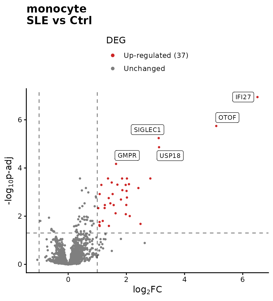

The 37 DEGs in monocytes go up in patients, and almost none goes down. The most significant ones (IFI27, SIGLEC1, USP18, IFI44L, OTOF) are interferon-stimulated genes: this is the interferon signature you saw in the previous lesson, now confirmed with statistics.

6.4 moDC

p_volcano_modc <- plot_volcano(de_classified$moDC, "moDC\nSLE vs Ctrl")
p_volcano_modc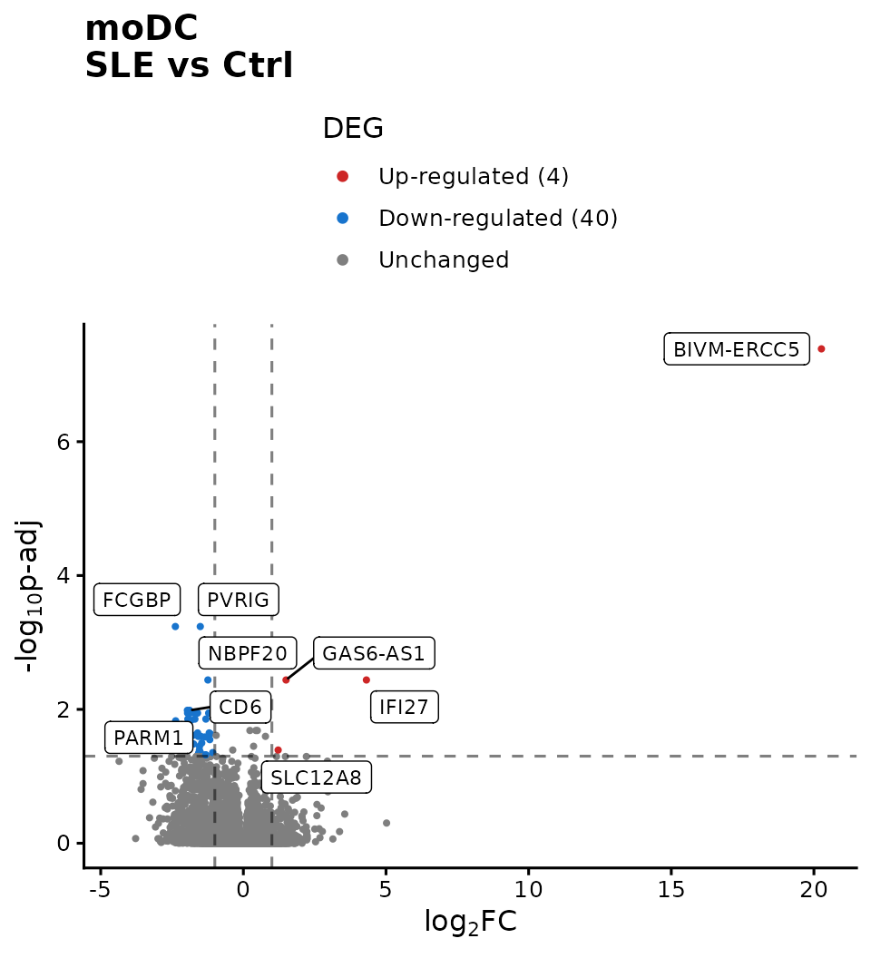

In moDC the pattern is reversed: genes that go down predominate (40) and only 4 go up. IFI27 still appears among those that go up.

Beware of extreme LFCs. BIVM-ERCC5 appears with an LFC close to 20 (a million times higher). Values like this are usually due to genes with almost zero reads in one of the groups: dividing by a nearly null number inflates the fold change. Before interpreting such a gene, check its normalized counts. DESeq2 offers lfcShrink() to obtain more realistic LFCs in these cases.

6.5 tolDC

p_volcano_toldc <- plot_volcano(de_classified$tolDC, "tolDC\nSLE vs Ctrl")
p_volcano_toldc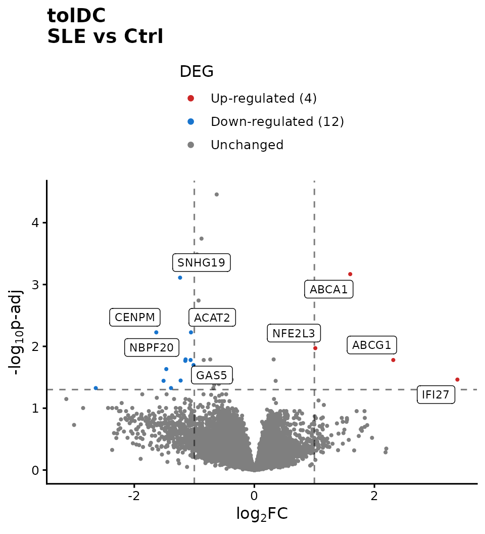

In tolDC there are 4 genes that go up and 12 that go down. Among those that go up are ABCA1 and ABCG1, cholesterol transporters: a hint of alterations in lipid metabolism, which we will explore in the next lesson.

up_genes <- lapply(de_classified, function(df) df$gene[df$Expression == "Up-regulated"])
down_genes <- lapply(de_classified, function(df) df$gene[df$Expression == "Down-regulated"])

Reduce(intersect, up_genes)                   # up in all three cell types
#> [1] "IFI27"
intersect(down_genes$moDC, down_genes$tolDC)  # down in moDC and tolDC
#> [1] "NBPF20"

c(up = length(unique(unlist(up_genes))), down = length(unique(unlist(down_genes))))
#>   up down 
#>   43   51

IFI27 goes up in all three cell types: it is a shared mark of lupus that persists even after differentiating the cells in vitro. In total there are 94 distinct DEGs (43 up and 51 down); in the next lesson we will find out which biological functions they have.

Challenge 2. Make a table with the LFC and padj of IFI27, USP18, and SIGLEC1 in the three cell types. In which one does each gene change the most?

Hint: bind_rows(de_results, .id = "Cell_type") joins the three tables into one.

Show solution

bind_rows(de_results, .id = "Cell_type") %>%
  filter(gene %in% c("IFI27", "USP18", "SIGLEC1")) %>%
  dplyr::select(gene, Cell_type, log2FoldChange, padj) %>%
  arrange(gene, Cell_type)
#>      gene Cell_type log2FoldChange         padj
#> 1   IFI27      moDC     4.31361093 3.635566e-03
#> 2   IFI27  monocyte     6.50565571 1.137584e-07
#> 3   IFI27     tolDC     3.38219155 3.445094e-02
#> 4 SIGLEC1      moDC    -0.42105695 9.995599e-01
#> 5 SIGLEC1  monocyte     3.11093020 5.737873e-06
#> 6 SIGLEC1     tolDC     0.04520298 9.765996e-01
#> 7   USP18      moDC     0.47562454 5.871915e-01
#> 8   USP18  monocyte     3.12316050 1.371820e-05
#> 9   USP18     tolDC     0.74759493 1.489008e-01

All three genes change the most in monocytes. IFI27 is the only one significant in all three cell types.

Challenge 3. Save the moDC DEGs to a CSV file, sorted by padj.

Hint: filter(), arrange(), and write.csv().

Show solution

de_classified$moDC %>%
  filter(Expression != "Unchanged") %>%
  arrange(padj) %>%
  write.csv("DEG_moDC_SLE_vs_Ctrl.csv", row.names = FALSE)

7. To finish: Figure 2 of the article

We bring everything together in Figure 2. The ComplexHeatmap heatmap is not a ggplot2 plot, so we first “capture” it as a graphical object with grid::grid.grabExpr() so that we can combine it with the others:

p_heatmap <- grid::grid.grabExpr(
  draw(top_annotation %v% heatmap_list,
       merge_legends = TRUE, annotation_legend_list = list(cell_legend),
       annotation_legend_side = "top", heatmap_legend_side = "top"),
  wrap.grobs = TRUE # keeps the drawing code so it can be redrawn inside the panel
)

right_panels <- plot_grid(
  p_markers,
  plot_grid(p_volcano_mo, p_volcano_modc, p_volcano_toldc,
            labels = c("C", "D", "E"), label_size = 18, nrow = 1),
  labels = c("B", ""), label_size = 18, ncol = 1, rel_heights = c(0.9, 1)
)

figure_2 <- plot_grid(p_heatmap, right_panels, labels = c("A", ""), label_size = 18,
                      nrow = 1, rel_widths = c(0.8, 1))
figure_2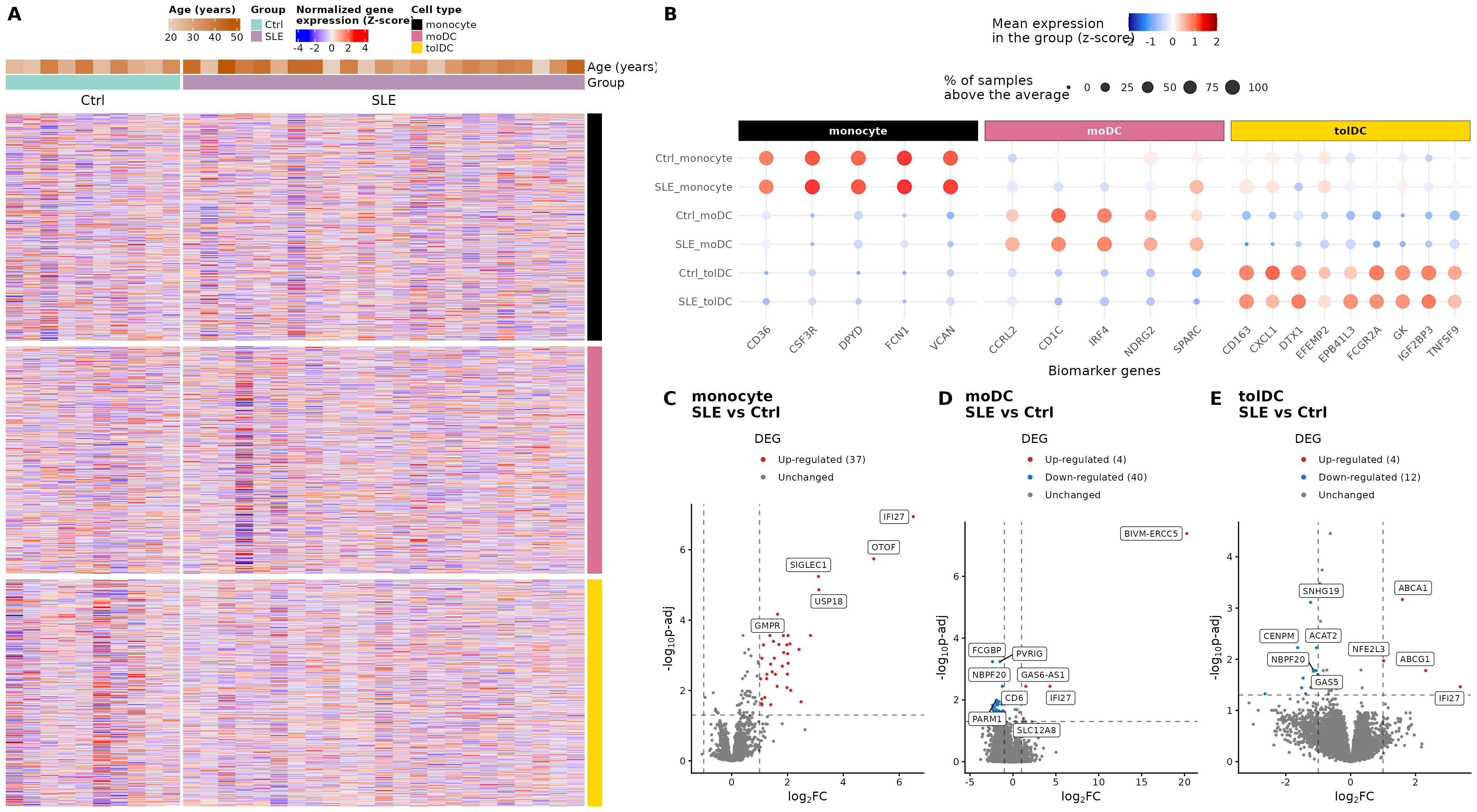


# Number of DEGs per cell type, for the figure caption
up_n   <- function(cell) sum(de_classified[[cell]]$Expression == "Up-regulated")
down_n <- function(cell) sum(de_classified[[cell]]$Expression == "Down-regulated")

Figure 2. Validation of the cell types and integrated transcriptomic profile between groups. (A) Heatmap of normalized gene expression, with genes in the rows and samples in the columns, for monocytes, moDC, and tolDC differentiated in vitro. The color scale represents the normalized counts as z-scores. At the top, the age and group of each volunteer (SLE or Ctrl) are annotated. (B) Biomarkers specific to each cell type. The color scale indicates the mean expression per group (z-score) and the dot size indicates the percentage of samples above the average of each gene. Each column is a biomarker of the cell type indicated above. (C–E) Volcano plots of the genes differentially expressed between groups in (C) monocytes (37 up and 0 down in SLE), (D) moDC (4 up and 40 down), and (E) tolDC (4 up and 12 down). DEGs were selected with |LFC| ≥ 1 and padj < 0.05, using the Wald test with Benjamini–Hochberg correction (FDR).

The original figure can be found in the article.

To save it in high resolution:

ggsave("Figure_2.png", figure_2, width = 20, height = 11, dpi = 300)

8. Checkpoint for the next lesson

You do not need to save anything: the package includes the result of this lesson under the same name, de_results (the DESeq2 results for the three cell types). The next lesson will start from there.

9. Summary

Step	Key function	What for?
Validate cell types	biomarker dot plot	Confirm the identity of the samples
Global view	`get_heatmap_mat()`, `create_heatmap()`	See the expression of all genes
Differential expression	`DESeq()`, `results()`	Test each gene: SLE versus Ctrl
Define DEGs	`padj < 0.05` and `\|LFC\| ≥ 1`	Keep reliable and relevant changes
Visualize	volcano plot	See the magnitude and significance of all genes
Compare cell types	`intersect()`	Find shared changes

Common beginner mistakes

Using pvalue instead of padj: with thousands of genes, hundreds would come out significant by chance.
Mixing all cell types in a single comparison: variation between cell types masks the differences due to lupus.
Interpreting a huge LFC without checking the counts: it may come from genes with almost no reads.
Not reporting the thresholds: the number of DEGs depends on them.
Thinking that “not a DEG” means “does not change”: with 10 controls, statistical power is limited.

10. Next steps

We have identified which genes change between patients and controls. The lesson Biological functions of differentially expressed genes addresses what functions they perform: through a functional enrichment analysis, we will associate the 94 DEGs with biological processes and pathways from Gene Ontology and Reactome.

To continue, click the Next lesson: Biological functions of DEGs button at the bottom of this page.

↑ Back to top

Session information

sessionInfo()
#> R version 4.6.2 (2026-10-29)
#> Platform: x86_64-pc-linux-gnu
#> Running under: Ubuntu 24.04.5 LTS
#> 
#> Matrix products: default
#> BLAS:   /usr/lib/x86_64-linux-gnu/openblas-pthread/libblas.so.3 
#> LAPACK: /usr/lib/x86_64-linux-gnu/openblas-pthread/libopenblasp-r0.3.26.so;  LAPACK version 3.12.0
#> 
#> locale:
#>  [1] LC_CTYPE=C.UTF-8       LC_NUMERIC=C           LC_TIME=C.UTF-8       
#>  [4] LC_COLLATE=C.UTF-8     LC_MONETARY=C.UTF-8    LC_MESSAGES=C.UTF-8   
#>  [7] LC_PAPER=C.UTF-8       LC_NAME=C              LC_ADDRESS=C          
#> [10] LC_TELEPHONE=C         LC_MEASUREMENT=C.UTF-8 LC_IDENTIFICATION=C   
#> 
#> time zone: UTC
#> tzcode source: system (glibc)
#> 
#> attached base packages:
#> [1] grid      stats4    stats     graphics  grDevices utils     datasets 
#> [8] methods   base     
#> 
#> other attached packages:
#>  [1] cowplot_1.2.0               ggrepel_0.9.8              
#>  [3] circlize_0.4.18             ComplexHeatmap_2.28.0      
#>  [5] lubridate_1.9.5             forcats_1.0.1              
#>  [7] stringr_1.6.0               dplyr_1.2.1                
#>  [9] purrr_1.2.2                 readr_2.2.0                
#> [11] tidyr_1.3.2                 tibble_3.3.1               
#> [13] ggplot2_4.0.3               tidyverse_2.0.0            
#> [15] DESeq2_1.52.0               SummarizedExperiment_1.42.0
#> [17] Biobase_2.72.0              MatrixGenerics_1.24.0      
#> [19] matrixStats_1.5.0           GenomicRanges_1.64.0       
#> [21] Seqinfo_1.2.0               IRanges_2.46.0             
#> [23] S4Vectors_0.50.3            BiocGenerics_0.58.1        
#> [25] generics_0.1.4              GeneExprLupusMx_0.1.0.9000 
#> 
#> loaded via a namespace (and not attached):
#>  [1] tidyselect_1.2.1    farver_2.1.2        S7_0.2.2           
#>  [4] fastmap_1.2.0       digest_0.6.39       timechange_0.4.0   
#>  [7] lifecycle_1.0.5     cluster_2.1.8.3     magrittr_2.0.5     
#> [10] compiler_4.6.2      rlang_1.3.0         sass_0.4.10        
#> [13] tools_4.6.2         utf8_1.2.6          yaml_2.3.12        
#> [16] knitr_1.52          labeling_0.4.3      S4Arrays_1.12.1    
#> [19] DelayedArray_0.38.2 RColorBrewer_1.1-3  abind_1.4-8        
#> [22] BiocParallel_1.46.0 withr_3.0.3         desc_1.4.3         
#> [25] ggh4x_0.3.1         colorspace_2.1-4    scales_1.4.0       
#> [28] iterators_1.0.14    cli_3.6.6           rmarkdown_2.32     
#> [31] crayon_1.5.3        ragg_1.5.2          otel_0.2.0         
#> [34] tzdb_0.5.0          rjson_0.2.23        cachem_1.1.0       
#> [37] parallel_4.6.2      XVector_0.52.0      vctrs_0.7.3        
#> [40] Matrix_1.7-6        jsonlite_2.0.0      hms_1.1.4          
#> [43] GetoptLong_1.1.1    clue_0.3-68         systemfonts_1.3.2  
#> [46] locfit_1.5-9.12     foreach_1.5.2       jquerylib_0.1.4    
#> [49] glue_1.8.1          pkgdown_2.2.1       codetools_0.2-20   
#> [52] shape_1.4.6.1       stringi_1.8.9       gtable_0.3.6       
#> [55] pillar_1.11.1       htmltools_0.5.9     R6_2.6.1           
#> [58] textshaping_1.0.5   doParallel_1.0.17   evaluate_1.0.5     
#> [61] lattice_0.23-1      png_0.1-9           bslib_0.12.0       
#> [64] Rcpp_1.1.2          SparseArray_1.12.3  xfun_0.62          
#> [67] fs_2.1.0            pkgconfig_2.0.3     GlobalOptions_0.1.4

Cell type validation, differential expression, and volcano plots

2026-10-31

Welcome

Lesson map

Glossary

1. Setup

Starting point

2. Step 1: are the cells what they claim to be?

3. Step 2: a global view with a heatmap

4. Step 3: differential expression with DESeq2

4.1 The question

4.2 Step by step with monocytes

4.3 The three cell types

5. Step 4: which genes change?

6. Step 5: volcano plots

6.1 How to read a volcano plot

6.2 A function for the three cell types

6.3 Monocytes

6.4 moDC

6.5 tolDC

7. To finish: Figure 2 of the article

8. Checkpoint for the next lesson

9. Summary

Common beginner mistakes

10. Next steps

Session information

Lesson 3: Differentially expressed genes between patients and controls

Cell type validation, differential expression, and volcano plots

2026-10-31

Welcome

Lesson map

Glossary

1. Setup

Starting point

2. Step 1: are the cells what they claim to be?

3. Step 2: a global view with a heatmap

4. Step 3: differential expression with DESeq2

4.1 The question

4.2 Step by step with monocytes

4.3 The three cell types

5. Step 4: which genes change?

6. Step 5: volcano plots

6.1 How to read a volcano plot

6.2 A function for the three cell types

6.3 Monocytes

6.4 moDC

6.5 tolDC

6.6 Which genes do the cell types share?

7. To finish: Figure 2 of the article

8. Checkpoint for the next lesson

9. Summary

Common beginner mistakes

10. Next steps

Session information